Jump to “A Little Bit More…” Solution
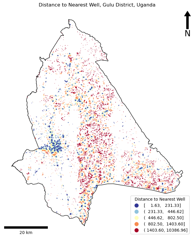
Initial wells: 3000
Filtered wells: 3000
Minimum distance to water in Gulu District: 2m.
Mean distance to water in Gulu District: 863m.
Maximum distance to water in Gulu District: 10,387m.
completed in: 0.36 seconds
done!
"""
Understanding GIS: Practical 3
@author jonnyhuck

Use spatial index to calculate the mean distance to a water supply in Gulu District

This version uses `shapely.STRtree` manually to demonstrate the process of creating a spatial index.

References:
	Guttman (1984):	https://dl.acm.org/doi/abs/10.1145/602259.602266
	Leutenegger(1997): https://apps.dtic.mil/sti/tr/pdf/ADA324493.pdf
	https://epsg.io/21096
	https://shapely.readthedocs.io/en/2.1.0/strtree.html
	https://geopandas.org/en/stable/docs/reference/api/geopandas.sindex.SpatialIndex.nearest.html
	https://matplotlib.org/3.1.1/api/_as_gen/matplotlib.pyplot.legend.html
    https://matplotlib.org/3.3.3/tutorials/intermediate/legend_guide.html

New Topics:
    Creating Functions
	Spatial Indexes with STRtree
	Iterating through a GeoDataFrame
"""
from math import sqrt
from shapely import STRtree
from time import perf_counter
from geopandas import read_file
from matplotlib.pyplot import subplots, savefig
from matplotlib_scalebar.scalebar import ScaleBar

def distance(x1, y1, x2, y2):
	"""
	* Use Pythagoras' theorem to measure the distance.
	* 	https://en.wikipedia.org/wiki/Pythagorean_theorem
	*
	* This is acceptable in this case because:
	*	- the CRS of the data is a local projection
	*	- the distances are short
	*  	- computational efficiency is important (as we are making many measurements)
	"""
	return sqrt((x1 - x2)**2 + (y1 - y2)**2)

# set start time
start_time = perf_counter()

# read in the shapefiles, and match up the CRS'
pop_points = read_file("../../data/gulu/pop_points.shp")
water_points = read_file("../../data/gulu/water_points.shp").to_crs(pop_points.crs)
gulu_district = read_file("../../data/gulu/district.shp").to_crs(pop_points.crs)

''' STAGE 1 - FILTERING THE DATA WITH A SPATIAL QUERY - EXTRACT ONLY WELLS INSIDE THE DISTRICT '''

# initialise an instance of an rtree Index object
idx = STRtree(water_points.geometry.to_list())

# get the one and only polygon from the district dataset (buffer by 10.5km to account for edge cases)
polygon = gulu_district.geometry.iloc[0].buffer(10500)	# buffer is from the 'A little more...' section

# report how many wells there are at this stage
print(f"Initial wells: {len(water_points.index)}")

# get the indexes of wells that intersect bounds of the district, then extract extract the possible matches
possible_matches = water_points.iloc[idx.query(polygon)]
print(f"Potential wells: {len(possible_matches.index)}")

# then search the possible matches for precise matches using the slower but more precise method
precise_matches = possible_matches.loc[possible_matches.within(polygon)]
print(f"Filtered wells: {len(precise_matches.index)}")


''' STAGE 2 - NEAREST NEIGHBOUR - find distance to nearest well for everybody'''

# rebuild the spatial index using the new, smaller dataset
idx = STRtree(precise_matches.geometry.to_list())

# declare array to store distances
distances = []

# loop through each population point
for id, house in pop_points.iterrows():

	# use the spatial index to get the index of the closest well
	nearest_well_index = idx.nearest(house.geometry)

	# use the spatial index to get the closest well object from the original dataset
	nearest_well = precise_matches.iloc[nearest_well_index].geometry.geoms[0]

	# store the distance to the nearest well
	distances.append(distance(house.geometry.x, house.geometry.y, nearest_well.x, nearest_well.y))

''' much faster vectorised replacement of the above loop via geopandas '''
# _, distances = precise_matches.sindex.nearest(pop_points.geometry, return_all=False, return_distance=True)

# calculate the mean
mean = sum(distances) / len(distances)

# store distance to nearest well
pop_points['nearest_well'] = distances

# output the result
print(f"Minimum distance to water in Gulu District: {min(distances):,.0f}m.")
print(f"Mean distance to water in Gulu District: {mean:,.0f}m.")
print(f"Maximum distance to water in Gulu District: {max(distances):,.0f}m.")

# finish timer
print(f"completed in: {perf_counter() - start_time} seconds")

# create map axis object
fig, my_ax = subplots(1, 1, figsize=(16, 10))

# remove axes
my_ax.axis('off')

# add title
my_ax.set_title("Distance to Nearest Well, Gulu District, Uganda")

# add the district boundary
gulu_district.plot(
    ax = my_ax,
    color = (0, 0, 0, 0),	# this is (red, green, blue, alpha) and means black, but transparent (alpha=0)
    linewidth = 1,
	edgecolor = 'black',	# this is just a shortcut for (0, 0, 0, 1)
    )

# plot the locations, coloured by distance to water
pop_points.plot(
    ax = my_ax,
    column = 'nearest_well',
    linewidth = 0,
	markersize = 1,
    cmap = 'RdYlBu_r',
    scheme = 'quantiles',
    legend = 'True',
    legend_kwds = {
        'loc': 'lower right',
        'title': 'Distance to Nearest Well'
        }
    )

# add north arrow
x, y, arrow_length = 0.98, 0.99, 0.1
my_ax.annotate('N', xy=(x, y), xytext=(x, y-arrow_length),
	arrowprops=dict(facecolor='black', width=5, headwidth=15),
	ha='center', va='center', fontsize=20, xycoords=my_ax.transAxes)

# add scalebar
my_ax.add_artist(ScaleBar(dx=1, units="m", location="lower left", length_fraction=0.25))

# save the result
savefig('out/3.png', bbox_inches='tight')
print("done!")
A Little Bit More…
This is the vectorised version:
"""
Understanding GIS: Practical 3 (Vectorised Alternative)
@author jonnyhuck

This approach uses higher-level functionality of geopandas to speed up the analysis
"""

from time import perf_counter
from geopandas import read_file
from matplotlib.pyplot import subplots, savefig
from matplotlib_scalebar.scalebar import ScaleBar

# set start time
start_time = perf_counter()

# read in the shapefiles, and match up the CRS'
pop_points = read_file("../../data/gulu/pop_points.shp")
water_points = read_file("../../data/gulu/water_points.shp").to_crs(pop_points.crs)
gulu_district = read_file("../../data/gulu/district.shp").to_crs(pop_points.crs)

''' STAGE 1 - FILTERING THE DATA WITH A SPATIAL QUERY - EXTRACT ONLY WELLS INSIDE THE DISTRICT '''

# get the one and only polygon from the district dataset (buffer by 10.5km to account for edge cases)
polygon = gulu_district.geometry.iloc[0].buffer(10500)

# construct the spatial index
water_points.sindex

# get the wells within the district
print(f"\nInitial wells: {len(water_points)}")
precise_matches = water_points.loc[water_points.within(polygon)]
print(f"Filtered wells: {len(water_points)}")


''' STAGE 2 - NEAREST NEIGHBOUR - find distance to nearest well for everybody'''

# ensure a new spatial index has been constructed on the new, smaller dataset
precise_matches.sindex

# use vectorised neares neighbour & distance calc
_, distances = precise_matches.sindex.nearest(pop_points.geometry, return_all=False, return_distance=True)
pop_points["nearest_well"] = distances

# output the result
print(f"Minimum distance to water in Gulu District: {pop_points['nearest_well'].min():,.0f}m.")
print(f"Mean distance to water in Gulu District: {pop_points['nearest_well'].mean():,.0f}m.")
print(f"Maximum distance to water in Gulu District: {pop_points['nearest_well'].max():,.0f}m.")

# finish timer
print(f"completed in: {perf_counter() - start_time:.2f} seconds")

# create map axis object
fig, my_ax = subplots(1, 1, figsize=(16, 10))

# remove axes
my_ax.axis('off')

# add title
my_ax.set_title("Distance to Nearest Well, Gulu District, Uganda")

# add the district boundary
gulu_district.plot(
    ax = my_ax,
    color = (0, 0, 0, 0),	# this is (red, green, blue, alpha) and means black, but transparent (alpha=0)
    linewidth = 1,
	edgecolor = 'black',	# this is just a shortcut for (0, 0, 0, 1)
    )

# plot the locations, coloured by distance to water
pop_points.plot(
    ax = my_ax,
    column = 'nearest_well',
    linewidth = 0,
	markersize = 1,
    cmap = 'RdYlBu_r',
    scheme = 'quantiles',
    legend = 'True',
    legend_kwds = {
        'loc': 'lower right',
        'title': 'Distance to Nearest Well'
        }
    )

# add north arrow
x, y, arrow_length = 0.98, 0.99, 0.1
my_ax.annotate('N', xy=(x, y), xytext=(x, y-arrow_length),
	arrowprops=dict(facecolor='black', width=5, headwidth=15),
	ha='center', va='center', fontsize=20, xycoords=my_ax.transAxes)

# add scalebar
my_ax.add_artist(ScaleBar(dx=1, units="m", location="lower left", length_fraction=0.25))

# save the result
savefig('out/3-vector.png', bbox_inches='tight')
print("done!")