In which we quantitatively examine the impact of our projection choices upon our maps and analyses.

Part 1

This week, we are going to have a go at defining the level of distortion in a map. As we all now know, map distortion is a major issue, but is something that is overlooked by most GIS users. Before that though, let’s do some preparation and have a think about the role of geometry in GIS.

Geometry for GIS

GIS is a multidisciplinary endeavour, and when focusing upon the computational aspects of GIS, it is important that you are reasonably comfortable with some aspects of basic (i.e., high school level) mathematics. Of key importance for vector-based GIS is geometry (concerned with the construction of shapes) and the associated field of trigonometry (specifically concerned with the construction of triangles).

In the lecture, we looked at a number of simple geometry tasks for measuring distance, direction, and point offset in Cartesian (projected) coordinate reference systems using Trigonometry.

A common problem in GIS that can be solved by Trigonometry is that of point offset: calculating a point at a given distance and direction from another point (e.g. what are the coordinates of a point 3km due east of my house).

Fortunately, this is also quite straightforward once you understand SOH CAH TOA. Let’s have another quick look at the image from the lecture:

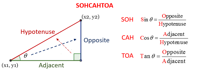
Here, we have the location of the first point \((x_1, y_1)\) and the length of the Hypotenuse (the red side of the triangle), which is the distance between the two locations. We need to calculate the coordinates of the second point, which is simply:

\(x_2 = x_1 + \Delta x\) (i.e., the length of the green side)

\(y_2 = y_1 + \Delta y\) (i.e., the length of the blue side)

Notice that we are using the symbol delta (\(\Delta\)) here, which is a Greek letter that is commonly used as a shorthand to mean difference in scientific descriptions. \(\Delta x\) therefore simply means the difference between the \(x\) coordinates.

Our task is then simply to calculate \(\Delta x\) (Adjacent, green) and \(\Delta y\) (Opposite, blue) and add them to \(x_1\) and \(y_1\) respectively!

Firstly, we need to decide which formula to use. For \(x\), we already have \(\theta\) and the length of the Hypotenuse (H) and we need the length of the Adjacent (A), so we need the CAH equation. Note the use of the theta symbol ( \(\theta\) ), which is another Greek letter that is used to mean the angle between the origin \((x_1,y_1)\) and destination \((x_2,y_2)\) - this is marked in the diagram above:

Or, in geographical terms:

Rearranging this to apply to our problem, we get:

Which we can then add to the coordinates of \(x_1\) to get the coordinates of \(x_2\):

Note that, as with all trigonometry functions, the cos() function in the Python math library expects angles to be in radians (a number in the range \((- \pi - \pi)\) ), so we must convert our direction from degrees (a number in the range \((0 - 360)\) ) to radians using the radians() function, also from the Python math library.

Make sure that you understand the above.

Use the SOHCAHTOA disgram above to work out the equivalent equation for \(x_2\)

Open week5/week5.py, paste in the below snippet and complete it using the knowledge from the above.

Run it to test.

from math import	# IMPORT NECESSARY FUNCTIONS HERE

def compute_offset(origin, distance, direction):
    """
    Compute the location of a point at a given distance and direction from a specified location using trigonometry
    """
    offset_x =	# COMPLETE THIS LINE
    offset_y =	# COMPLETE THIS LINE 
    return (offset_x, offset_y)

# this code tests whether your function works correctly
origin = (345678, 456789)
destination = compute_offset(origin, 1011, 123)	# move 1011m in a direction of 123 degrees 
print("CORRECT!!" if (int(destination[0]), int(destination[1])) == (345127, 457636) else f"INCORRECT!! Error: {(int(destination[0])-345127, int(destination[1])-457636)}")

If all has gone to plan, then you should get the message CORRECT!!. Otherwise, you will get a message like INCORRECT!! Error: (-139, -108), where the values are the error (to the nearest metre) in the x and y coordinate respectively.

Make sure you keep going until you get it right - you need this in Part 2!

You can learn more about Trigonometry operations in Python on the Trigonometry page of this website.

Part 2

Assessing Map Distortion

One of the reasons that people do not tend to calculate the level of distortion in a map (aside from the lack of easily available tools to do so) is that there is not a very clear consensus on how this should be achieved. As we saw in the lecture, approaches to the measurement of map distortion fall into two broad classes: local (or infinitesimal scale), and global (or finite scale) measures. Local measures (which include Tissot’s Indicatrix) allows the assessment of how distortion changes across a map, but do not provide the basis for comparison of map projections or evaluation of suitability. For this reason, Frank Canters proposed a set of global metrics that can provide a single figure for distortion on a given map in his 2002 book “Small Scale Map Projection Design”.

I adopted these methods in a recent publication (Huck 2025), which provided a detailed assessment of map projection distortion in the production of globes. For the interested, additional descriptions of these methods can be found in Canters et al. (2005) (pages 2-5) and Gosling & Symeonakis (2020) (pages 267-268).

Read the Distortion Assessment section of Huck (2025) so that you have an idea of the method we will be using this week.

A clear set of measures

As you can see in the paper, we will calculate a metrics for each of the three types of map distortion:

• \(E_P\) (Ep): Distance Distortion
• \(E_S\) (Es): Shape Distortion
• \(E_A\) (Ea): Areal Distortion

Note: this week, we will break with convention and not use snake_case in some cases, in order to match variable names to mathematical notation. This is not unusual in mathematical applications of Python.

Based on these measures, we can clearly understand the level of distortion for a given map, which is an extremely desirable thing to do, especially when we are trying to decide which CRS we should use to present and/or analyse our data!

Motivation

Rather than assessing map projections for globes (which is quite niche), we will assess them for the production of a standard topographic map, much like those produced by Ordnance Survey in the UK (and available to us in digital format from Digimap). These maps are designed using the British National Grid map projection, which is conformal (based on Transverse Mercator), as this facilitates the use of a compass for navigation. However, because it is also a local projection, the levels of area and distance distortion are sufficiently low that they are regularly used for measuring distances and areas as well.

Not that long ago, Geographical Information Scientists in the UK would routinely use OS maps as background maps for almost everything, partly because there were few alternatives available . In recent years, however, web maps (such as OpenStreetMap or ESRI Maps) have begun to be included in GIS software, providing a more easily accessible (if generally poor quality) base map. This is particularly evident in ArcGIS Pro, in which a new “blank” map is pre-populated with an ESRI web map by default.

The problem with this, of course, is that web maps are projected using the “Web Mercator” projection, which is a global conformal map projection, and therefore exhibits large amounts of distortion, especially towards the poles. This default behaviour therefore means that many GIS workspaces also end up projected into Web Mercator, which is an unsuitable choice for almost all GIS operations!

To illustrate the scale of the problem (pun intended…), see the example below, where you can drag a circle and the outline of Greenland around on the map. See how their size and shape change with latitude (and think what that would do to your measurements!):

Using the methods described above, we can avoid issues like this by calculating the level of each type of distortion in a given map using the approach described in Huck (2025), and thus make informed decisions about our choice of map projection.

This is what we will learn to do today, through an experiment in which we are using projected data to calculate the surface area of Ice in Iceland.

Getting Started

Loading the datasets

Open the "../../data/natural-earth/ne_10m_admin_0_countries.shp" file as a GeoDataFrame and load it into a variable called world. Remember to add the necessary import statement at the top of your code.

Extract the Iceland row from the GeoDataFrame (the ISO code is ISL) and store it in a variable called iceland.

Open the ../../data/iceland/gis_osm_natural_a_free_1.shp file as a GeoDataFrame and load it into a variable called land_cover.

Extract all rows where land_cover.fclass == "glacier", and store the result in a varable called ice

We need to begin by extracting the bounds of Iceland. We will do this using the .total_bounds property of the iceland GeodataFrame. This is useful, as it accounts for the bounds of all parts of the country (which is useful for countries that are made up of multiple components, such as the UK as we saw last week).

Add the below snippet to calculate the bounds of Iceland, which uses variable expansion to extract them into 4 separate variables (rather than a Tuple of 4 items)

# get the bounds of the country
minx, miny, maxx, maxy = iceland.total_bounds

Add a print() statement to test the bounds, if all has gone to plan they should look something like this:

-24.539906378999945 63.39671458500004 -13.502919074999909 66.56415436400005

Defining our Geodesic model and CRSs

Fundamentally, each of the three measures (\(E_P\), \(E_S\), \(E_A\)) are calculated by simply comparing a measure of each property (distance, shape, area) taken using a on the ellipsoid, to one drawn using the selected projection. The closer that each projected circle is to the ellipsoidal version, the less distortion there is, and vice-versa. Simple!

For the purposes of this project, we will use the WGS84 Datum as our ellipsoidal model, which is a pretty solid choice for working at a global scale (it is the one that the GPS uses). Let’s get started:

Initialise a pyproj Geod object set to WGS84 with the below snippet (remember to add the necessary import statement at the top of your code):

# set the geographical proj string and ellipsoid (should be the same)
geo_string = "+proj=longlat +datum=WGS84 +no_defs"
g = Geod(ellps='WGS84')

Now we need to define the CRS that we will be comparing. We will use three:

• Web Mercator: a widely used global conformal projection (to illustrate the problems with this widely, but wrongly, used projection)
• Eckert IV: a widely used global equal area projection (the phenomena in which we are interested is the surface area of the ice)
• A local equal area projection of your own design choice (to illustrate the difference between the local and global projection)

Let’s store our projections as proj strings in a list of dictionaries, so that we can easily include some information about them as well:

# create a list of dictionaries for the projected CRS' to evaluate for distortion
projections = [
    {'name':"Web Mercator", 'description':"Global Conformal",   'proj':""},
    {'name':"Eckert IV",    'description':"Global Equal Area",  'proj':""},
    {'name':"", 'description':"Local Equal Area",   'proj':""}
]

Add the above snippet to your code

Fill in the missing proj strings for Web Mercator and Eckert IV

Fill in the third entry using a local equal area projection that you create using the Projection Wizard (remember to give it an appropriate name too)

If all went to plan, you will probably end up with a projection based on Albers’ Conic projection. As per the model we stored in the g variable, we will use the WGS84 datum for all projections.

Calculating Distortion for each Projection

The broad approach that we will take here is:

For each projection:
	Build a pyproj Transformer
	For each of 1000 random circles:
		Calculate areal and shape distortion indices
	Loop 1000 times:
		Calculate distance distortion indices
	Calculate the final area, shape and distance distortions values

To help us with this, we will loop through our list of dictionaries (projections) using the enumerate() function. As we saw in class, this adds a second loop variable to act as a counter for each iteration of the loop. enumerate()is one of the built-in functions in Python, which means that it does not require an import statement. See here:

# loop through each CRS
for ax_num, projection in enumerate(projections):

Note the use of variable expansion here - enumerate() provides the count variable first, then the current item in the collection, so in this case ax_num is the counter (containing the values 0, 1, 2) and projection will contain the dictionary containing the current projection information. This is similar to how we get the index value (row number) and row of data when we use GeoDataFrame.iterrows().

Make sure that this makes sense and then add the above snippet to your code.

Add a print statement so that you can see the counter and object change at each iteration of the loop

The first thing to do inside the loop code block is to create a pyproj.Transformer object, which enables you to transform coordinates from one CRS to the other, and vice-versa.

Edit your import statements so that you are importing CRS and Transformer from pyproj

Add the below snippet to create a Transformer object that can transform coordinates between your two CRS’:

# initialise a PyProj Transformer to transform coordinates
transformer = Transformer.from_crs(CRS.from_proj4(geo_string), CRS.from_proj4(projection['proj']), always_xy=True)

Note how we are extracting the proj value from the projection dictionary with projection['proj']. Also note how this takes in two pyproj.CRS objects to define the transformation, and also that we need to force it to use coordinates in the order Longitude-Latitude (x, y). This is because some libraries and software prefer to do things in the order Latitude-Longitude. This can easily lead to many errors if you get them mixed up - so I always try to stick with the conventional x-y (Longitude-Latitude) approach!

Now we have our Transformer ready to go, we can start assessing our distortion.

Add the function call from the snippet below as the next line in your code

# calculate the distortion
evaluate_distortion(g, transformer, minx, miny, maxx, maxy, 10000, 1000000, 1000)

Now, create the function using the below def statement - remember that functions go below the import statements, but above the main code

def evaluate_distortion(g, transformer, minx, miny, maxx, maxy, minr, maxr, sample_number, vertices=16):

Note how we have

Note how we have set a default value of 16 for the vertices argument. This means that we could call this function without setting a value for vertices, and the Python Interpreter would just set it to 16 for us!

Add a default values of 1000 for sample_number

Note: From here until we get to the return statement, the majority of the up-coming code should be placed inside the evaluate_distortion function, unless otherwise specified!

Assessing Area and Shape Distortion

Random Sampling

In order to assess area and shape distortion across the whole map, we will draw 1,000 circles of random size at random locations. Here, we will create them first and then loop through them.

In order to select 1,000 random locations within the study area, we need to do nothing more complicated than selecting 1,000 random \(x\) coordinates (longitude) and 1,000 random \(y\) coordinates (latitude); each within the bounds that we defined earlier. We will then draw a circle (with a random radius) at each of these 1,000 locations.

We will achieve this using numpy, which is a maths package for Python. numpy contains many functions to help us create sets of random numbers - we will use one called uniform(), which draws random numbers from a uniform distribution. This sounds a bit complicated, but simply means that all numbers between the supplied bounds are equally likely to be returned. This as opposed to a normal distribution, for example, where numbers near the middle of the range would be more likely to be returned than those near the bounds. Because we don’t want any bias towards any parts of our study area over others, uniform() is the correct choice.

Here is how to collect our random \(x\) coordinates:

from numpy.random import uniform

# calculate the required number of random locations (x and y separately) plus radius
xs = uniform(low=minx, high=maxx, size=sample_number)

This will return a list with a length equal to size, in which each element is a random number between low and high. Here you can see that we are using keyword arguments, where each argument is named (you have seen these before in the .plot() function, for example). These are exactly the same as normal arguments, they are just convenient for when a function has a lot of optional arguments, as it means that you only have to specify values for the arguments that you are interested in, and can accept the default values for the others.

Add the above snippets to your code (the import at the top and the function call in your evaluate_distortion() function)

Now add two more lines to get the random ys (latitudes, ranging from miny to maxy) and rs (random circle radii, ranging from minr to maxr)

Print some values from your resulting lists to see if they are as expected

In order to construct our circles, we will use the approach described by Canters et al. (2005):

For each [circle] 16 positions along its perimeter are calculated, corresponding to
azimuthal angles of 0,22.5,45,..., defined from the centre of the circle. By 
projecting each position along the circle's outline in the plane a polygon with 16
vertices is obtained.

In order to achieve this, we will need to prepare a list of azimuths (directions) in which the centre point will need to be offset in order to construct our circle.

Add the below snippets to your code in order to define your 16 directions using arange() (very similar to the already familiar range(), but it permits the use of non-integer numbers) - here we are achieving this by asking for a list of numbers from 0-360 at intervals of 22.5 (³⁶⁰/₁₆, or ¹/₁₆ of a circle)

from numpy import arange

# offset distances
forward_azimuths = arange(0, 360, 22.5)

We will not actually construct our circles just yet - but now we have prepared everything that we need to do so.

Looping through our random points and radii

Now that we have everything in place for our random circles, we need to loop through the random data that we have created. As we have three lists that we want to loop through (xs, ys, rs), we are going to use the zip() function in Python to allow us to loop through them all at once. zip() is another built-in function, so does not require an import statement. See here:

# create two lists
list_1 = [1, 2, 3, 4, 5]
list_2 = ['A', 'B', 'C', 'D', 'E']

# zip and extract using variable expansion
for x, y in zip(list_1, list_2)
	print(x, y)

…which would return:

1 A
2 B
3 C
4 D
5 E

make sure that you understand zip() - if you need a little more info, you can get it here.

Define three empty lists called area_indices, shape_indices and distance_indices

Add a for statement to loop through xs, ys and rs using zip() - call the loop variables x, y and r

Now each random circle is defined by x, y and r in each iteration of the loop - great!

Building our random circles

In order to assess our circles for distortion, we need to construct them using two different approaches:

• construct the circle on the ellipsoid and then transform it to projected coordinates
• construct the circle using projected coordinates

Comparing these two circles then lets us assess the level of distortion.

Here is how we do it:

We can construct our circle by simply offsetting our point along the ellipsoid by a given distance and direction (forward azimuth). As you might remember from Week 2, we have an equation that will do this for us called the Forward Vincenty Equation, and that is available to us thanks to pyproj as g.fwd():

# construct a circle around the centre point on the ellipsoid
lons, lats = g.fwd([x]*vertices, [y]*vertices, forward_azimuths, [r]*vertices)[:2]

As with the g.inv() function that you will remember from Week 2, g.fwd() returns three sets of values (one or more longitudes, one or more latitudes and the back azimuth). Because we are not interested in the back azimuth, we can ignore it using list slicing, where we extract only the first two elements from the returned collection using [:2].

Unlike the example from Week 2, here we are passing in lists as each of the arguments (rather than single values). This is a convenient feature of the g.fwd() function, which means that it can either take in single values as arguments (and return single values), or lists as arguments (and return lists). The only snag here is that we only have one list (forward_azimuths), as x, y and r all remain the same.

Fortunately, Python has a simple solution for us - we can put the single value in a list (by surrounding it with square brackets), and then multiply that by our desired length, which will duplicate the one value as many times as we multiply by:

bunch_of_fives = [5]*10
print(bunch_of_fives)

…which gives:

[5, 5, 5, 5, 5, 5, 5, 5, 5, 5]

Handy!

Note: though [5]*10 works, 10*[5] doesn’t - so make sure you get it the right way around (with the list first)!

Make sure that you fully understand the g.fwd() statement above (including the list multiplication), then add it to your loop.

Next, we want to loop through our lists of ellipsoidal coordinates (lons and lats) and project them, which we simply do by passing them to transformer.transform() using zip() and List Comprehension for elegance and efficiency. We will then store the area of this circle (which we calculate by building the coordinates into a shapely.Polygon and then using the .area property).

Note that direction='FORWARD' refers to the fact that we are transforming from geographical to projected coordinates. direction='BACKWARD' would be from projected to geographical.

from shapely.geometry import Polygon

# project the result, calculate area, append to the list
e_coords = [ transformer.transform(lon, lat, direction='FORWARD') for lon, lat in zip(lons, lats) ]

# get the area of the resulting circle
ellipsoidal_area = Polygon(e_coords).area

Make sure that you understand the above snippet and then add it to your code

Now we have the area for our circle constructed on the ellipsoid, we will do exactly the same thing for a circle constructed on the projection plane. To do this, we simply need to transform the x, y coordinate (the centre of the circle), and then calculate the 16 points around the edge of the circle using the compute_offset() function that you created in Part 1. Again, we will use list comprehension to do this in an elegant and efficient manner:

# transform the centre point to the projected CRS
centre_x, centre_y = transformer.transform(x, y, direction='FORWARD')

# construct a circle around the projected point on a plane, calculate area
planar_area = Polygon([ compute_offset((centre_x, centre_y), r, az) for az in forward_azimuths ]).area

Make sure that you understand the above snippet and then add it to your code

Reflect on the difference between the above two snippets and make sure that you understand how these different approaches result in different geometries with different areas. If you don’t understand - ask!

Calculating the area and shape distortion values

The ultimate goal of this loop is that we will end up with a lists of values that we can slot into the Equation from Huck (2025) to calculate area and shape distortion. Now we have the area of our two circles (one ellipsoidal, one projected), we are in a position to do this - here is what we want to calculate for each pair of circles:

where: \(a\) is the area distortion value for this sample, \(S_i\) is the ellipsoidal area, \(S'_i\) is the projected area.

Pipes surrounding a number (e.g., |x|) means the absolute value of \(x\), which is the distance of the number from 0. This simply means that for positive numbers it is the number itself, and for negative numbers it is the number without the sign (i.e., the positive equivalent). It is handled in Python by the abs() function, which is built-in and so does not need to be imported from a library. For example:abs(3) = 3, whereas, abs(-5) = 5.

Complete the below snippet using the equation above and and add it to your code

area_indices.append(  )

We now need to do the same for shape distortion. This one is based on the below, which works out the absolute difference in the expected length of each of the 16 ‘spokes’ (as a proportion of the total length of all of the spokes) - if it is a perfect circle then they will all be \(\frac{1}{16}\) and the index will be \(0\). If it is not a perfect circle, then the number will be \(>0\). Note that we are once again using List Comprehension here:

# get radial distances from the centre to each of the 16 points on the circle
ellipsoidal_radial_distances = [ hypot(centre_x - ex, centre_y - ey) for ex, ey in e_coords ]

# get the absolute proportional difference between the expected and actual radial distance for each 'spoke'
shape_distortion = [abs((1 / vertices) - (d / sum(ellipsoidal_radial_distances))) for d in ellipsoidal_radial_distances]

Add the above snippet to your code to get a list of 16 absolute proportions, then get the sum of that list and append it to your shape_indices list.

Now exit the code block for your loop and check the length of your area_indices and shape_indices lists - they should both be equal length (your chosen sample number!)

The final step is to turn those lists of indexes into a single value for the map, which is simply a matter of slotting them into the other part of the equation from Huck (2025), e.g., for area this would be:

Where: \(m\) is the sample size (sample_size) and \(A\) is the list of \(a\) values generated above (area_indices). \(\sum_{i=0}^m A_i\) is like the equation equivalent of a for loop - it simply means “sum of all of the values in \(A\) (using the counter variable \(i\), which stops when it reaches \(m\))”. The eagle-eyed amongst you will see that this is simply a matter of calculating the mean of the list of values!

Apply the equation to both lists (making sure that you are outside the loop!!) and store the result in variables called Ea and Es.

Print them out - do they match with your expectations? (Think about which projection(s) you are evaluating…)

Calculating Distance Distortion

OK, we have done our area and shape distortion metrics, now we just need one for distance distortion. Our distance distortion metric uses the same equation as the one that we used for area. The only difference is that \(S_i\) and \(S'_i\) refer to the distance between a pair of random points (ellipsoidal and projected respectively), as opposed to the area of a randomly generated circle.

As you might imagine, the process is therefore also quite similar, let’s get started:

Use range() to make a for loop that will run sample_number times - we will not be using the loop variable directly, so you can call it _

Inside the loop, use two calls to uniform() to generate two random locations within the map bounds. Store the resulting coordinates in variables called xs and ys

Add a temporary print() statement to make sure that you are getting coordinates as expected

We now need to calculate the distance between the two locations across the ellipsoid. Ordinarily, we would expect to use the g.inv() function to do this, just like we did in Week 2. This time, however, we are going to use the g.line_length() function, which does pretty much the same thing - the only differences are that it does not also return the forward and back azimuths (which we do not need) as well as the distance, and it takes the coordinates as two arrays (one of x coordinates, one of y coordinates), which is convenient as it is the format in which we already have the coordinates (xs and ys):

# calculate the distance along the ellipsoid
ellipsoidal_distance = g.line_length(xs, ys)

Add the above snippet to your loop to calculate the distance

Add a temporary print() statement to make sure that the results are expected

Next, we need to undertake the same measurement exercise for the projected points:

Add two transformer.transform() statements to project both of your random locations. Store the results in two variables called origin and destination

Calculate the distance between the two points using hypot() (as you did earlier) and store the result in a variable called planar_distance

Finally, we just need to calculate the distance distortion index value and append it to the distance_indices - this is exactly the same as you did with area, see the equation below:

where: \(d\) is the distance distortion value for this sample, \(S_i\) is the ellipsoidal distance, \(S'_i\) is the projected distance (remember abs() too).

That is all that we need for our loop, you are now ready to calculate your metric!

Outside of the loop, calculate \(E_P\) (remember, it is exactly the same as it was for \(E_A\)!)

Finally…

Add the following return statement to your function…

# return the three distortion the measures
return Ep, Es, Ea

…and then modify your call to the evaluate_distortion() function (don’t add a second one!!) so that it matches the below snippet - this way it stores the three returned values into the corresponding variables using variable expansion:

# calculate the distortion
Ep, Es, Ea = evaluate_distortion(g, transformer, minx, miny, maxx, maxy, 10000, 1000000, 1000)

Now we have updated the return statement and function call, our evaluate_distortion() function is complete - we will now return to working in the main body of code (i.e., outside the code block for the function).

Calculating the Ice Area

Now that we have our distortion values, it would be useful to put those numbers in context by seeing what impact it has on our area calculation.

# calculate ice area
ice_area_km2 = ice.to_crs(projection['proj']).geometry.area.sum() / 1000000

Note that here we are dividing the value by 1,000,000 (1000 \(\times\) 1000) to convert the units from \(m^2\) (the CRS units) to \(km^2\), which is a more appropriate metric for reporting the area of such large features.

Make sure that you understand the above snippet and then add it to your script

Then add the following snippet to check your results:

# report to user
print(f"\n{projection['name']} ({projection['description']})")
print(f"   {"Distance distortion (Ep):":<26}{Ep:.6f}")
print(f"   {"Shape distortion (Es):":<26}{Es:.6f}")
print(f"   {"Area distortion (Ea):":<26}{Ea:.6f}")
print(f"   {"Ice Area:":<26}{ice_area_km2 / 1000:,.0f} km sq.")

Note the use of the <26 format specifier for the labels, which simply means left aligned (<) and 26 characters long (26) - this helps to align the results into a nice table format.

Run your code

You should expect to see something approximately like the below. Note that the results will be slightly different each time because you are using a different set of random circles and lines each time. Methods like this are called stochastic methods (as opposed to deterministic, which means you will get exactly the same result every time). The trick with stochastic methods is simply to make sure that you have enough circles to make the difference between runs very small (you can experiment with this using your code - fewer circles will give bigger differences between runs, and vice versa!):

Web Mercator (Global Conformal)
   Distance distortion (Ep): 0.405402
   Shape distortion (Es):    0.054654
   Area distortion (Ea):     0.700697
   Ice Area:                 69,004 km sq.

Eckert IV (Global Equal Area)
   Distance distortion (Ep): 0.133295
   Shape distortion (Es):    0.227497
   Area distortion (Ea):     0.002553
   Ice Area:                 12,829 km sq.

Albers Conic (Local Equal Area)
   Distance distortion (Ep): 0.000070
   Shape distortion (Es):    0.000490
   Area distortion (Ea):     0.000351
   Ice Area:                 12,882 km sq.

You can see now how the three projections differ in their relative levels of distortion, as well as the impact that this has on the result (the value for ice area). Note that even the two Equal Area projections have different area results (i.e., the distortion is not zero)! This is important to realise, and you can read more about this problem in equal-area map projections in the article: All Equal-Area Map Projections Are Created Equal, But Some Are More Equal Than Others by Usery and Seong (2001).

You will also notice that the Web Mercator Projection is not as conformal as you might expect - you can read more about this issue in Battersby et al (2014), and on the Wikipedia page.

Have a think about how neither the Web Mercator nor Exkert IV, both of which are widely-used map projections, do exactly what we expected.

In this context, reflect on the way that you select map projections in your other modules. This is why this kind of understanding is so valuable - as you now have the power to actually check!

Making a map

To complete the practical, we need a map to illustrate the differences in the three projected versions of Iceland.

As ever, I will not walk you through each element of this in as much detail, but you should make sure that you fully understand it.

In this case, we are going to make a figure that contains three maps, and we will be populating it as we go, so we will have our plotting code scattered throughout our script, rather than at the end like it has been in the previous weeks.

First, add the below function at an appropriate location - this is just a convenience function that ensures our output maps are square (which is useful for keeping everything aligned in our layout)

def make_bounds_square(ax):
    """
    * Adjust the bounds of the specified axis to make them for to a square
    """
    # get the current bounds
    ax_bounds_x = ax.get_xlim()
    ax_bounds_y = ax.get_ylim()

    # get the width and height
    ax_width = ax_bounds_x[1] - ax_bounds_x[0]
    ax_height = ax_bounds_y[1] - ax_bounds_y[0]
    
    # if width is larger, expand height to match
    if ax_width > ax_height:
        buffer = (ax_width - ax_height) / 2
        my_axs[axx][axy].set_ylim((ax_bounds_y[0] - buffer, ax_bounds_y[1] + buffer))
    
    # if height is larger expand width to match
    elif ax_width < ax_height:
        buffer = (ax_height - ax_width) / 2
        my_axs[axx][axy].set_xlim((ax_bounds_x[0] - buffer, ax_bounds_x[1] + buffer))

Next, add the following snippet before your projections loop (so it will run once, before the loop starts):

# create a 2x2 figure
fig, my_axs = subplots(2, 2, figsize=(10, 10), constrained_layout=True)
fig.suptitle('How much Ice is in Iceland?\n', fontsize=20)
text = ""

Now add this snippet at the start of your projections loop (so it will run once per projection, before the existing contents of the loop)

# get x and y position of current axis
axx = ax_num // my_axs.shape[0]
axy = ax_num % my_axs.shape[0]

Next, add this snippet at the end of your projections loop (so it will run once per projection, after the existing contents of the loop)

# append text for figure
text += f"{projection['name']+":":<13} $E_p={Ep:.4f}$  $E_s={Es:.4f}$  $E_a={Ea:.4f}$\n\n"

# disable axis, add title
my_axs[axx][axy].axis('off')
my_axs[axx][axy].set_facecolor('#000000')
my_axs[axx][axy].set_title(f"{projection['name']} ({projection['description']})\nIce area: {ice_area_km2:,.0f} km sq.")

# plot iceland
iceland.to_crs(projection['proj']).plot(
    ax = my_axs[axx][axy],
    color = "#b2df8a",
    edgecolor = '#33a02c',
    linewidth = 0.2,
    )

# plot ice
ice.to_crs(projection['proj']).plot(
    ax = my_axs[axx][axy],
    color = "#e6f5f9",
    edgecolor = "#e6f5f9",
    linewidth = 0.1,
    )

# add scalebar
my_axs[axx][axy].add_artist(ScaleBar(dx=1, units="m", location="lower right"))

# adjust the plot bounds to fit a square
make_bounds_square(my_axs[axx][axy])

Finally, append the following snippet to the end of your file (so it will run once, after everything else has completed)

# disable axis on the empty axis
my_axs[1][1].axis('off')

# manually draw a legend to the empty axis
my_axs[1][1].legend([Patch(facecolor='#e6f5f9', edgecolor='#e6f5f9', label='Glacier')], ['Glacier'], loc='lower right')

# add north arrow to empty axis
x, y, arrow_length = 0.9, 0.3, 0.15
my_axs[1][1].annotate('N', xy=(x, y), xytext=(x, y-arrow_length),
    arrowprops=dict(facecolor='black', width=3, headwidth=9),
    ha='center', va='center', fontsize=16, xycoords=my_axs[1][1].transAxes)

# add the results to the empty axis - monospace font ensures table alignment
my_axs[1][1].text(0.1, 0.4, text, fontfamily='monospace')

# save the result
savefig('out/5.png', bbox_inches='tight')
print("done!")

Now run your code to test it

If all has gone to plan, you should have something like this:

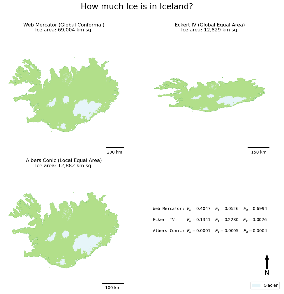
When considered alongside the figures, the maps really help you to see the patterns of distortion, particularly in the shape (look at Eckert IV!) and area/distance (look at the difference in the scale bars between Web Mercator and your local Albers Conic!).

Make sure that you can see the patterns of the results reflected in the maps

Making your code into a library

The last thing that we will do this week is to convert our code so that we can call it as a library from another Python Script. This is surprisingly easy to do, all that you need is to take the code that is not inside a function and put it inside the following if statement:

if __name__ == "__main__":
  # code goes here

This looks a little odd - but is a pretty fundamental (and very common) line to find in Python code. It is simply a conditional statement checking whether or not a variable called __name__ contains the value "__main__". The way it works is explained here, but in essence, __name__ is a variable that gets populated automatically by Python when a module or package is imported. Normally, this is set to the name of the Python file itself, except if the file is run directly (which means it is the top level code, i.e., the first to run), in which case it is set to the String "__main__".

Testing whether or not the __name__ variable is set to __main__ therefore tells us whether or not the script has been run directly (in which case the code block will run), or has been imported as a library (in which case it won’t). Simple!

This approach then gives you the following basic structure for a Python script:

# imports 

# functions

if __name__ == "__main__":
	# rest of your code

Add a if __name__ == "__main__": statement to your code so that nothing will happen if it is imported (apart from the functions being created).

Add a new file called test.py to your week5 directory and add the following. Save and run to test it. If it works you should get the a similar answer (accounting for the randomness) as you got from your other script (make sure that the countries are the same, of course…)!

from geopandas import read_file
from week5 import evaluate_distortion
from pyproj import Geod, CRS, Transformer

# set the projected CRS to evaluate for distortion
proj_string = "+proj=eck4 +lon_0=0 +x_0=0 +y_0=0 +datum=WGS84 +units=m +no_defs"  # Eckert IV (Equal Area)

# set the geographical proj string and ellipsoid (should be the same)
geo_string = "+proj=longlat +datum=WGS84 +no_defs"
g = Geod(ellps='WGS84')

# load the shapefile of countries and extract country of interest
world = read_file("./data/natural-earth/ne_10m_admin_0_countries.shp")

# set country using country code
country = world.loc[world.ISO_A3 == "ISL"]

# get the bounds of the country
minx, miny, maxx, maxy = country.total_bounds

# initialise a PyProj Transformer to transform coordinates
transformer = Transformer.from_crs(CRS.from_proj4(geo_string), CRS.from_proj4(proj_string), always_xy=True)

# calculate the distortion
Ep, Es, Ea = evaluate_distortion(g, transformer, minx, miny, maxx, maxy, 10000, 1000000, 1000)

# report to user
print(f"{"Distance distortion (Ep):":<26}{Ep:.6f}")
print(f"{"Shape distortion (Es):":<26}{Es:.6f}")
print(f"{"Area distortion (Ea):":<26}{Ea:.6f}")

Now you can import that functionality into your script any time you like, simply copy the week5.py file into your working directory and use it as above!

We have done this because these functions are not included in any mainstream GIS systems or Python libraries, so it will be very useful for you to be able to uses these to evaluate the level of distortion in your future maps.

A little more…

If you want to keep going, see if you can implement the alternative areal distortion metric (\(r\)) given by Gosling & Symeonakis (2020) (equation 3, page 268). This is an example of a classic Intersection over union operation, which is simply achieved by creating the polygons of the two versions of your circle (which you already do) and then using the .intersection() and .union() topological operators from shapely to get the values (see Week 2 or the Handy Hints page)

where:

• \(K\) = The circle created on the ellipsoid and then projected (\(S\) in the above)
• \(L\) = The circle created using a projection (\(S'\) in the above)
• \(\cap\) intersect (it looks like an n, as in intersection)
• \(\cup\) union (it looks like a u, as in union)

\(K \cap L\) would therefore be the area of the polygon created by an intersection between polygon \(K\) and polygon \(L\), whilst \(K \cup L\) is the area of the union of the two polygons.

As with the shape distortion metric, you would calculate \(r\) for each circle in your random sample, and then get the mean value to give you the overall \(r\) value.

How does it compare to the areal distortion metric that we used in the practical?