4. Understanding Generalisation
A quick note about the practicals...
Remember that coding should be done in Spyder using the understandinggis virtual environment. If you want to install the environment on your own computer, you can do so using the instructions here.
You do not have to run every bit of code in this document. Read through it, and have a go where you feel it would help your understanding. If I explicitly want you to do something, I will write an instruction that looks like this:
This is an instruction.
Remember that we are no longer using Git CMD. You should now use GitHub Desktop for version control.
Don't forget to set your Working Directory to the current week in Spyder!
Shortcuts: Part 1 Part 2
In which we examine the coastline paradox, and discover that distance is even more confusing than we previously thought
Welcome to Week 4
Two weeks ago, we calculated the length of the border between two countries, and learned all about how our model of the shape of the Earth (flat, spherical, ellipsoidal) affects the distance that we end up with. We have also learned that the CRS and Datum/Ellipsoid can affect this too. However, as we will see below, there are other forces at play as well, and measuring the length of features such as a border, coastline or river is still this is not quite as simple as it first appears, even once you account for all of the above - this is because we also need to consider scale and generalisation in the dataset.
To understand this, we will be examining a generalisation algorithm called the Visvalingam-Whyatt algorithm, which was developed by my good friend Prof. Duncan Whyatt (Lancaster University) in 1991 as part of his PhD. It has been described as ‘more effective ‘ than the older though perhaps better known ‘Douglas-Peucker ‘ algorithm, and much of this is down to the intuitive way in which it progressively removes the points that cause the least-perceptible change in the shape of the feature.
We will examine this algorithm in the context of the Coastline Paradox, whilst simultaneously discovering that the concept of distance is, once again, much more complex than we previously thought. Specifically, we will use the skills that we developed over the past three weeks in order to determine the length of the coastline of mainland Great Britain and see how it varies with generalisation. The critical takeaway here is that all data are generalised to some extent, so we can’t ever just ignore this!
Before we get stuck in this week, there are a few more fundamentals of Python with which I would like you to become familiar. The first of these is Conditional Statements…
Part 1
Conditional Statements in Python
Simply, conditional statements are used to allow your script to make decisions; essentially deciding whether or not a particular block of code should run.
The best known conditional statement is the if statement, which simply tests whether or not a condition evaluates to either True or False. This may sound simple, but it is a powerful tool, allowing the code to make decisions based upon the values associated with certain variables.
The components of an if statement are very simple, with the minimum requirement being simply:
if condition:
	# this code only runs if the condition was true
e.g.
if name == 'Jonny':
    print('Hi Jonny!')
The section between the if and : can be any statement that evaluates to True or False (a Boolean value) - this can be achieved using comparison operators (e.g. >, <=, == etc.), or a function that returns a Boolean value, such as the tests for topological relationships that we looked at last week. For example:
if point.within(france_geom):
  print('Bonjour!')
NB: Note the difference between the assignment operator = (which assigns a value to a variable), and the equality operator == (which tests whether or not two values are equal)!
You can have as many if statements in a row as you like, and they will all be evaluated each time the code runs, even if one of them turns out to be true:
if name == 'Jessica':
    print('Hi Jessica!')
if name == 'Sneha':
    print('Hi Sneha!')
if name == 'James':
    print('Hi James!')
Because we know that if name == 'Jessica', then name is definitely not also going to == 'Sneha' or == 'James', then we can make the process more efficient by using an elif statement (which means ‘else if’) that will only be evaluated if the previous statement evaluates to False:
name = 'Sneha'

if name == 'Jessica':		# this will be tested, and is False
    print('Hi Jessica!') # this will therefore NOT run

elif name == 'Sneha':		# this will be tested, and is True
    print('Hi Sneha!') 	# this will therefore run

elif name == 'James':	 	# this will NOT be tested, as we already know the answer
    print('Hi James!')  # this will therefore NOT run
Which would result in:
Hi Sneha!
Sometimes, this is important for efficiency (as above), but in other cases it is essential to ensure that the code is correct. Consider this for example:
if population > 1000000000:
    print('billions of people live here')
if population > 1000000:
    print('millions of people live here')
if population > 1000:
    print('thousands of people live here')
If the population is, say, 2 billion people, then all three conditions will evaluate to True, and all three statements will print out, which would be incorrect! Using the below version with elif (“else if”) solves this problem, because the statement will end after one of the conditions evaluates to True.
if population > 1000000000:
    print('billions of people live here')
elif population > 1000000:
    print('millions of people live here')
elif population > 1000:
    print('thousands of people live here')
What would happen if the order of the tests were reversed? Would it still work?
However, now imagine a population of 100, which would print out nothing!
We could add more options, but another alternative is to add an else statement to the end of that, which will run only if all of the above conditions evaluate to False:
if population > 1000000000:
    print('billions of people live here')
elif population > 1000000:
    print('millions of people live here')
elif population > 1000:
    print('thousands of people live here')
else:
    print('this has a small population')
Pretty simple right? Enabling your code to make decisions is a very useful tool, and one that you will likely use quite a lot!
More on Lists in Python
A few weeks ago, I introduced you to lists in Python. Before we move on, I am going to just give you a bit more information about things that you can do with lists. Specifically, these are some of the functions that you can use to edit lists:
| Function | Description |
|---|---|
list.append(x) |
Add an item to the end of the list. |
list.insert(i,x) |
Insert an item at a given position. The first argument is the index of the element before which to insert, so a.insert(0, x) inserts at the front of the list. |
list.remove(x) |
Remove the first item from the list whose value is x. It is an error if there is no such item. |
list.pop() list.pop(i) |
Remove the item at the given position in the list, and return it. If no index is specified, a.pop() removes and returns the last item in the list. |
list.index(x) |
Return the index in the list of the first item whose value is x. It is an error if there is no such item. |
list.count(x) |
Return the number of times x appears in the list. |
list.sort() |
Sort the items of the list. |
list.reverse() |
Reverse the elements of the list, in place. |
More details on lists in python can be seen here. As ever, you do not need to memorise these, merely know that they exist and where to look them up if you need them!
You should also know that you can concatenate lists using the addition operator (+) - just like you can with strings. So, for example:
list_a = [1, 2, 3]

list_b = ['A', 'B', 'C']

list_c = list_a + list_b

print(list_c)
Which will print:
[1, 2, 3, 'A', 'B', 'C']
Simple!
Preparing our data…
Before we get stuck into generalisation, we first need some data to generalise. Just like Mandelbrot, we will use the coastline of Great Britain.
However, this requires us to actually get the coastline of Great Britain out of our countries dataset…
Open
week4/week4.pyand paste in the below code snippetComplete the incomplet line of code by adding the missing definition string for the British National Grid and the missing query to extract the row that refers to the UK (hint: see week 2 - the ISO code for the UK is
GBR).
from geopandas import read_file

# open a dataset of all countries in the world
world = read_file("../../data/natural-earth/ne_10m_admin_0_countries.shp")

# extract the UK, project, and extract the geometry
uk = world[(  )].to_crs(  ).geometry.iloc[0]	# COMPLETE THIS LINE

# report geometry type
print(f"geometry type: {uk.geom_type}")
Note how the middle line of code is doing three things, whch could equally be done in three separate lines:
- filtering the dataset to get the UK row
- Projecting the result to British national grid
- extracting the geometry (first the column with
geometry, then the geometry itself with.iloc[0])
Make sure that the above makes sense and you can see all of the parts working together
Run the code
Did you get it? If so you should have had something like this:
geometry type: MultiPolygon

As you can see, this snippet is accessing the .geom_type property of the Geometry object, in order to report the geometry type that it stores (Point, LineString, Polygon etc.). Knowing the type of an object is important for many types of analysis (e.g. there is no point checking whether or not something is within a LineString, as this would be impossible!). It is therefore good practice to combine the .geom_type property with a conditional statement to ensure that your code is robust in cases where the analysis depends upon the geometry type of our dataset, e.g.:
if uk.geom_type == 'MultiPolygon':
  # anything in here would only run if the geometry is a MultiPolygon
For example, note that here we have a MultiPolygon rather than simply a Polygon - this is because the United Kingdom is composed of a number of islands, as well as territories that are not attached to the mainland (e.g. Northern Ireland). As with MultiLineString and MultiPoint, a MultiPolygon is simply a version of the geometry type that can hold more than one geometry in the same feature. Underneath, a MultiPolygon simply contains a list of individual Polygon objects, which can be accessed using the .geoms property.

Whilst this is a good representation of the UK, it is not ideal for what we are doing today - we will therefore extract mainland Great Britain from the uk MultiPolygon before we go any further. We can do this by looping through each Polygon (accessed via the .geoms property) and then calculating the area of each one using the .area property. However, if we were dealing with a Polygon object (of which there are several in this dataset) rather than a Multipolygon, then the .geoms property would not be available, and our code would fail:
AttributeError: 'Polygon' object has no attribute 'geoms'
We must therefore be careful to check the .geom_type before we do any analysis that relies upon it. Here is the code to check this and then extract the largest polygon from it:
from sys import exit
# quit the analysis if we are dealing with any geometry but a MultiPolygon
if uk.geom_type != 'MultiPolygon':
  print("Geometry is not a MultiPolygon, exiting...")
  exit()
This is an example of Look Before You Leap programming - checking that something is not going to cause an error before we try it, and ending the script (with exit() if so). We will come back to this in more detail in the coming weeks. Take particular note of:
-
the use of the
.geom_typeproperty in the conditional statement to ensure that we only undertake this analysis on geometry of the typeMultiPolygon. - the use of
!=(not equal to) in order to print a message and quit the program gracefully (exit()). This could also be achieved just as efficiently with anifstatement that only ran the analysis if it was aMultiPolygon- it is just slightly clearer this way as it means that the rest of the script doesn’t need to be indented. - In most cases you will want to have different approaches for multiple geometry types, using a set of
if-elif-elsestatements. Here we are only implementing a solution forMultiPolygons.
Make sure the above snippets make sense to you, when they do, add them to your code in suitable locations.
Now that we are sure we have a MultiPolygon, we need to work out which of its constituent Polygons is the largest:
# initialise variables to hold the coordinates and area of the largest polygon
biggest_area = 0
coord_list = []

# loop through each polygon in the multipolygon and find the biggest (mainland Great Britain)
for poly in uk.geoms:

	# if it is the biggest so far
	if 	# COMPLETE THIS LINE

		# store the new value for biggest area
		biggest_area = poly.area

     # store the coordinates of the polygon
		          = list(poly.boundary.coords)	# COMPLETE THIS LINE (look at the variables that you defined before the loop)
Read over the above and make sure that it makes sense
In particular, take note of:
- the use of the
.geomsproperty of theMultiPolygonobject to access (and iterate over) the underlying list ofPolygonobjects - the use of
list(poly.boundary.coords)statement, this extracts the boundary of thePolygon(as in boundary and interior from Understanding Topology…) using the.boundaryproperty, and then extracts the list of coordinate pairs describing that boundary using the.coordsproperty. Finally, this is converted to a list using thelist()function.
Once you understand it, add the above snippet to your code, and complete the two incomplete lines
Use some
print()statements to test that you have successfully populatedbiggest_areaandcoord_list(it is better to just print the length of this one withlen()).
If all has gone to plan, your value for biggest_area should be approximately 218,535,916,642m2; whereas coord_list will simply be a long list of coordinate pairs. Note that if your biggest_area is a little different (say, within 1% of my value), then this is probably due to floating point rounding on your machine (i.e., how many decimal places it can store in a number). The fewer decimal places, the less precise the coordinates, and the further away from the target the result will be! This is just another of the many reasons why we can’t think of results from computational processes as being perfectly correct.
That’s all for now - back to the lecture!
Part 2
Preparing for Generalisation
Remember to remove or comment out any old
print()statements that you don’t need anymore once you have used them to check that your code works! You should keep doing this yourself (particularly in assessments) - I won’t keep reminding you…
The Visvalingam-Whyatt algorithm operates by reducing a line to a defined number of nodes (points along the line) - in computational geometry applications, these are often called vertices, but here we will use nodes, as this is the term that Visvalingam and Whyatt used. As in the original paper, this number is normally given as the percentage of nodes that will be removed. We need to translate that into the number of nodes that we want in the resulting line, which we can easily do with the below snippet:
# set the percentage of nodes that you want to remove
SIMPLIFICATION_PERC = 98
# how many nodes do we need?
n_nodes = int(len(coord_list) / 100.0 * (100 - SIMPLIFICATION_PERC))

# ensure that there are at least 3 nodes (minimum for a polygon)
if n_nodes < 3:
	n_nodes = 3
Note how we are using a conditional statement to ensure that we end up with a minimum of three nodes - this is important, because fewer than three nodes cannot make a polygon.
Also note how I have used a variable in capital letters (SIMPLIFICATION_PERC) to hold the input number. This way, if we want to change the level of simplification, we can simply edit the variable, and the result will be changed. This is much more convenient than if we had just hard-coded the number 98 at several locations throughout our code, which would have been a pain to update (and could easily lead to mistakes - remember: Don’t Repeat Yourself!). This is a good example of elegant coding - which is useful for when we start to think about assessments… Variables like this (i.e. ones defining settings or other definitions that will not be changed as the code runs) are often presented in capitals to mark them out (though this is not essential).
Add the above snippets to your code at suitable locations (the setting variable right up at the top, just below the
importstatements, so that it is easy to find and change should you want to do so).
The Visvalingam-Whyatt Algorithm
Rather than just adding the Visvalingam-Whyatt algorithm directly into our code, we are going to use a function. This is good for two reasons:
- It makes our code neater, as it keep the code for a discrete job separate from the rest
- It means that we can call the function multiple times if we wish, rather than having to copy and paste code for the whole algorithm each time (DRY!).
Both of the above make your code more elegant, and easier to maintain. As above, elegance will attract greater marks in the Assessments…
Use a
defstatement to create an empty function calledvisvalingam_whyatt()with two arguments:node_listandn_nodes. Remember that functions should be above the rest of your code, but below the import statements.
node_list will be the list of points that need to be simplified, and n_nodes will be the number of nodes that should be returned in the simplified list.
I have already explained how the Visvalingam-Whyatt algorithm works, but let’s start with a brief recap:
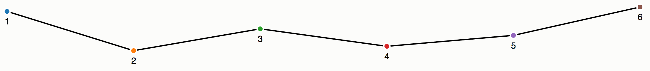
The Visvalingam-Whyatt algorithm works by computing the area of triangles that are formed by each triplet of nodes along a line. The area of a triangle formed from a node and the node to the left and right of it is referred to as the effective area of that node. The algorithm simply continuously removes the node with the smallest area until the required number of nodes (often defined by a percentage) remain. For example (and borrowing some images from Mike Bostock’s explanation), here is a line made up of six nodes:
In the Visvalingam-Whyatt algorithm, the first and last point always stay where they are (both because they are important, and because they do not have nodes on both sides of them with which to make a triangle). For all of the nodes except the end ones, however, we can make triangles and calculate the effective area:
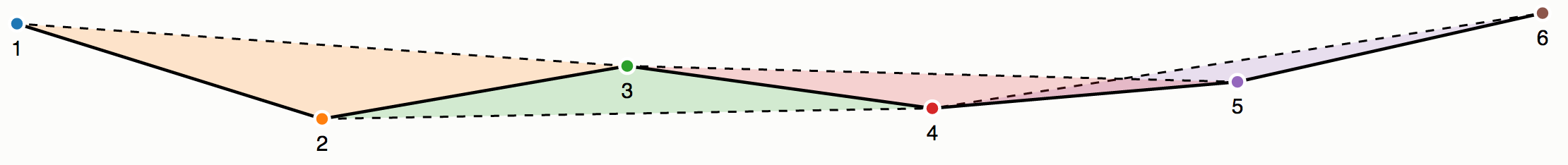
Of those 4 triangles, the purple one (associated with node 5) has the smallest area (i.e. node 5 has the smallest effective area). As such, it is removed by the algorithm, and triangle 4 is re-calculated:
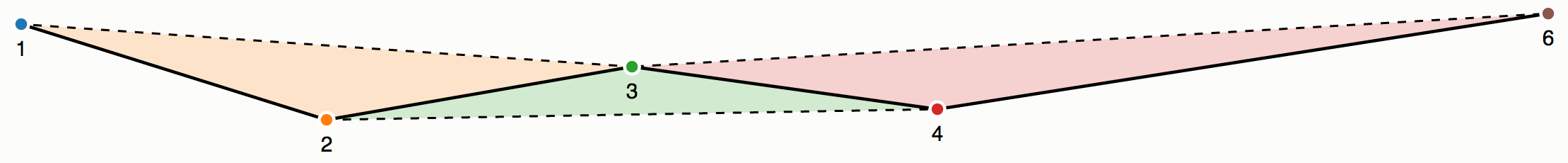
Now, the green triangle is the smallest, meaning that node 3 has the smallest effective area, and so this one is removed next, and so on, until only the endpoints remain:
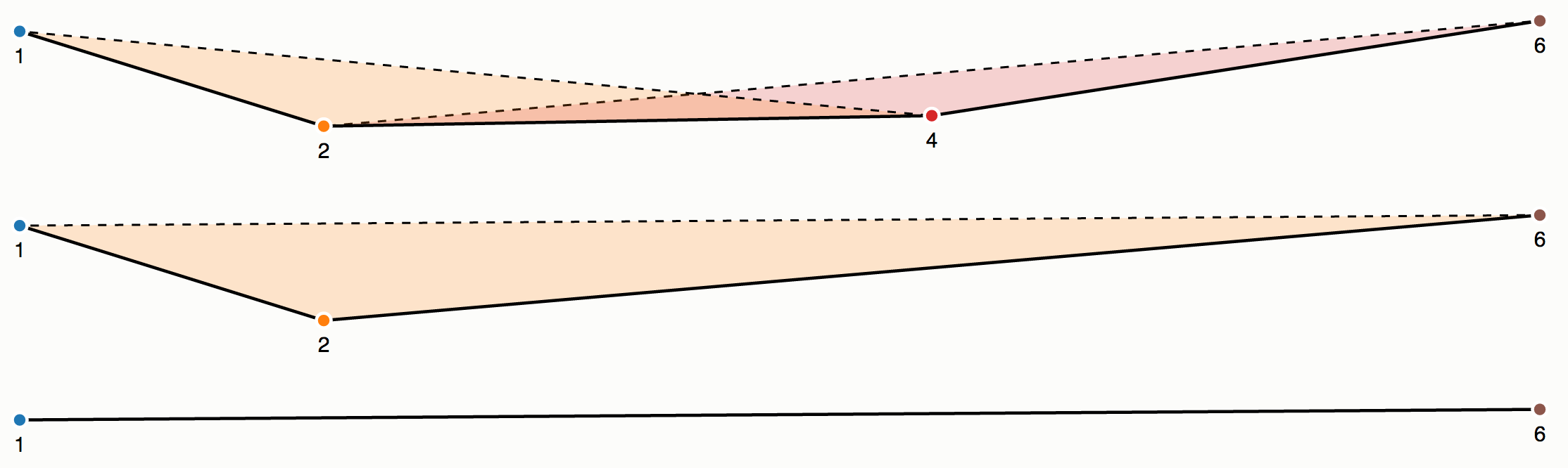
Quite simple right? This is why it is so popular, you can calculate the simplification really quickly, and the results are comparatively good-looking compared to some of the other (slower) algorithms.
Our code is going to do exactly this, except that it will stop at the point that we have the desired number of nodes remaining (rather than keeping going until we have only a straight line left).
Effective Area
As you can see, the main thing that we need to be able to do in order to perform Visvalingam-Whyatt Simplification is work out the Effective Area of each point, which is the area of a triangle formed by the point and both of its neighbours:
We can’t do much more in our visvalingam_whyatt() function before we establish how to calculate the Effective Area of a point - so before we do anything else, lets have a go at that.
There is a set formula for calculating the area of a triangle from its coordinates called Heron’s Formula (click for details). It looks a bit complicated at first, but it is simply a matter of calculating the perimeter of the triangle, dividing it by two (giving the semi-perimeter), and then plugging it into the formula. A valid alternative to this would be to use the coordinates to produce a Polygon object and then simply use its .area property; but we are here to really understand what we are doing, not simply get the answer, and this approach should be more efficient too!
def get_effective_area(a, b, c):
	"""
	* Calculate the area of a triangle made from the points a, b and c using Heron's formula
	* 	https://en.wikipedia.org/wiki/Heron%27s_formula
	"""
	# calculate the length of each side
	side_a = distance(b[0], b[1], c[0], c[1])
	side_b = distance(a[0], a[1], c[0], c[1])
	side_c = distance(a[0], a[1], b[0], b[1])

	# calculate semi-perimeter of the triangle (perimeter / 2)
	s = (side_a + side_b + side_c) / 2

	# apply Heron's formula and return
	return sqrt(s * (s - side_a) * (s - side_b) * (s - side_c))
Add the above snippet as a new function (remember that this is a separate function, so should be just below your
importstatements at the top of the file, and NOT inside yourvisvalingam_whyatt()function)You will also need your
distance()function from last week to make this work - add that too - and remember to include any associatedimportstatements!
It is appropriate to separate get_effective_area() and distance() into functions for the same reasons as visvalingam_whyatt(). Crucially - these are blocks of code that we will be calling many times from several parts of our script, so should definitely be in a function to avoid repetition, and make it easy to edit in the future.
Pseudocode
A popular way of describing an algorithm is using pseudocode (pronounced ‘soo-doh-code’). This is a useful way of communicating algorithms to other programmers, because it is easy to understand, and (crucially) does not require you to be able to understand any particular programming language in order to use it.
Basically, pseudocode is nothing more than writing an algorithm out in an easily readable way, but structured as if it was code (making it easy to read and understand for other programmers). You can see an example of pseudocode in the Wikipedia article for the Douglas-Peucker algorithm (an alternative algorithm for line simplification).
There are no fixed rules for how pseudocode should look, it’s just down to the author to make it as readable as possible. Some will look almost like a programming language (like in the Douglas-Peucker example above), others will be little more than indented English language (like the example below).
Here is the Visvalingam-Whyatt algorithm represented as pseudocode, adapted from what was written in the original 1993 paper to make it fit our needs:
Compute the effective area of each point

Delete the end points and store them in a separate list

REPEAT

	Find the point with the least effective area and call it the current point

	Delete the current point from the list

	Recompute the effective area of the two adjoining points

UNTIL The desired number of points remain
Note how they have used REPEAT and UNTIL to open a loop and define when it should finish, and tabs to indicate the code block inside the loop.
Read through the above description and pseudocode and make sure that you understand it before you move on.
Back to the Visvalingam-Whyatt Algorithm…
Now go back to your visvalingam_whyatt() function. As you can see in the pseudocode, the first thing that we need to do is work out the effective area of each point in the dataset. However, we cannot work this out for the end points of the line, because they do not have a point on either side of them, and so cannot make a triangle.
We will therefore use the range() function that we covered in week 2 to loop from the second item in the node_list (index 1) to the second-to-last item (index len(node_list)-1). In this way, we skip out the end points, and can safely calculate our areas.
For each point included in our loop, we will then calculate the effective area and store both the point and the effective area in a dictionary, which we will store in a list called areas. As we saw in the lecture dictionaries are lists of key and value pairs in the form key:value. Our dictionary will have two keys:
'point': this will store the coordinates of the point'area': this will store the effective area of the point
Add the below snippet to your
visvalingam_whyatt()function.Complete the incomplete line by adding the node to the left of
node_list[i]as the first argument and the node to the right ofnode_list[i]as the third argument (this is quite intuitive if you think about it)
# loop through each node, excluding the end points
areas = []
for i in range(1, len(node_list)-1):

  # get the effective area
  area = get_effective_area(  , node_list[i],  )	# COMPLETE THIS LINE

  # append the node and effective area to the list
  areas.append({"point": node_list[i], "area": area})
Make sure that you understand this snippet, in particular how we are using
range()to loop through only part of the list, and how we are constructing a list of dictionaries
Once the loop has completed, we will simply add in the end points (with a ‘fake’ effective area of 0) to the list using the .insert() function at index locations 0 (the start of the list) and len(areas) (the end of the list). See Part 1 or here for more information how this function works.
Add the below snippet after your loop has completed (think about the indentation…):
# add the end points back in at the start (0) and end (len(areas))
areas.insert(0, {"point": node_list[0], "area": 0})
areas.insert(len(areas), {"point": node_list[len(node_list)-1], "area": 0})
Add the below function call to call the
visvalingam_whyatt()function at the appropriate location.
Note that you do not yet return anything from the function, so simplified_nodes will be equal to None for now (as nothing gets put in it) - this is simply to make the function run so that we can test it as we write!
# remove one node and overwrite it with the new, shorter list
simplified_nodes = visvalingam_whyatt(coord_list, n_nodes)
Back inside the
visvalingam_whyatt()function, add aprint()statement to compare the length (len()) of theareaslist to the length ofnode_list. If you have done everything right, then they should be the same!
Now we have stored the values for each node in a dictionary, we can retrieve the values by putting the key name (with speech marks) into square brackets after the variable name (so for the element with index i in areas the coordinates would be accessed using areas[i]['point']; and the effective area would be accessed using areas[i]['area'].
Eliminating Nodes
Now we know the effective area for each of our points, we can loop through and start removing nodes. To do this, we need to repeatedly find the node with the smallest effective area and remove it from the list, until we are left with the desired number of nodes.
Because we will be removing items from the list, we will first want to take a copy of it. This is because we want to keep the original as well so that we can compare them later. As you saw in the lecture, simply using the assignment operator (=) on lists, dictionaries, or any other immutable object would simply produce a reference to the same location in memory, and so any changes that we made to our new copy would also be reflected in the original.
To avoid this, we must make a shallow or deep copy of our object using the .copy() or .deepcopy() member functions of the List object respectively. Note that for other objects that do not have these functions built in, they are also available in a Python library called copy.
As we saw in the lecture, the difference between the two is down to whether or not the contents of the new list are also copied (as in a deep copy), or are simply references (as in a shallow copy). In our case, we are simply going to be removing items from our list (rather than editing items within it), so a shallow copy will suffice. As you would expect, this is a more time and memory efficient option, so should be preferred to deep copy where possible.
To make a shallow copy of your list, add the below snippet to your code:
# take a copy of the list so that we don't edit the original
nodes = areas.copy()
From this point, we can now do what we like to nodes (our shallow copy), without affecting areas (the original).
We now want to start the process of repeatedly removing nodes until we have reduced them to the desired number. To achieve this, we will use a different type of Loop Statement: a while loop.
This is a bit like a for loop, but keeps going until a certain condition is met, as opposed to looping through each member of a list. In this case, we want to loop continually until the number of nodes that we have equals the value of the n_nodes variable. We therefore write this as:
# keep going as long as the number of nodes is greater than the desired number
while len(nodes) > n_nodes:
Everything inside the block of this while loop will therefore run again and again until the number of nodes in nodes is no longer greater than n_nodes (i.e., when we have the correct number remaining!).
Add the above snippet to your code - be careful to make sure that you are keeping track of your indentations - this should be inside your
Visvalingam_whyatt()function.
Warning! Do not run your code at this stage - as we are not yet removing any nodes from the list, the length will never become equal to n_nodes, so the code will run infinitely!!
Now, according to the pseudocode, we need to work out which point has the smallest effective area.
Using the list of hints below, create a
forloop that finds the point innodeswith the smallest effective area and store the index of the point in a variable callednode_to_delete..
Remember to determine your algorithm before getting started!
Hints:
- This is almost the same procedure as when you found the largest feature in the UK in Part 1.
- The only difference with finding the smallest thing in a list is that you will need to start your variable at a very large number (rather than
0). Python has a handy tool for this job, which represents infinity (meaning that any number will be smaller than it; just like any positive number is greater than0). You can set a variable to infinity like this:min_area = float("inf"). min_area = float("inf")will need to be inside thewhileloop, but outside of theforloop, as it will need to be reset each time you remove a node.- As with before, we need to ignore the end points here, as they do not have an effective area - so make sure that you loop from
1tolen(nodes)-1, just like we did before! - Remember that you have already calculated the effective areas, and stored them in the
'area'key of each element innodes(so to retrieve the effective area of the node with indexi, you can simply usenodes[i]['area']. - Remember to use
print()statements to check what your code is doing while you are writing it - as a rule of thumb it is good to check each line as you write it to avoid errors! - Bear in mind that you have already done the majority of this (or very similar) today - so this shouldn’t be too much of a stretch to do this if you take the time to think about it!
Once you have the index of the node with the smallest effective area, you can remove it from the list with a simple pop() statement (see Part 1 for more info):
# remove the current point from the list
nodes.pop(node_to_delete)
Add the above snippet to your code
Hint: be careful to get the indent in the right place - this should be outside your for loop (as we don’t want to remove every single node), but inside your while loop (as we want to remove one each iteration - otherwise the loop will run infinitely!).
Now we have added the code to remove the node, we can safely test the last stage of our code:
At this point, add a
print()statement to print out how many elements are in thenodeslist then run it, you should be able to see it counting down as it runs!
Next, according to the pseudocode, we just need to re-calculate the effective area for the point to the left and right of the point that we just removed. In practice, this will actually be the one to the left of node_to_delete and the one at the location of node_to_delete as everything to the right of node_to_delete will have moved one place to the left when we deleted it):
Look at C in the list below, it is in position 3:
1  2  3  4  5
A, B, C, D, E
To the left is B (position 2) and right is D (position 4).
However, if we now DELETE C:
1  2  3  4
A, B, D, E
Then B remains in position 2, but D is in position 3, having replaced C.
Therefore, we need to re-calculate the effective area for node_to_delete-1 (left), and node_to_delete (right). In the latter case, we need to make sure that we do not fall off the end of the list using an if statement.
Add the below snippet to your function and complete the missing first arguments in the calls to
get_effective_area()
# recalculate effective area to the left of the deleted node
nodes[node_to_delete-1]['area'] = get_effective_area(   , nodes[node_to_delete-1]['point'],    )	# COMPLETE THIS LINE

# if there is a node to the right of the deleted node, recalculate the effective area
if node_to_delete < len(nodes)-1:
	nodes[node_to_delete]['area'] = get_effective_area(   ,   ,   )		# COMPLETE THIS LINE
Run your code again and make sure that it is still counting down as expected. (Remember to remove the
print()statement when you have completed this - it is just for testing, and you don’t want it there forever!!)
Finally, we just need to return the points. For this, we will use list comprehension to extract only the coordinates (and not the effective areas, which we no longer need) from the nodes list.
# extract the nodes and return
return [ node['point'] for node in nodes ]
Add the above snippet to your code - note that this is the
returnstatement, so should only be called after thewhileloop has completed (i.e. think about your indentation…)
We could, of course, do this with a normal loop and an append() function as per the below, but as we saw in the lecture, that would be slower and less elegant:
# extract the nodes and return
out = []
for node in nodes:
  out.append(node['point'])

return out
As a rule, use list comprehension to construct a list where possible
You should now have a perfectly serviceable implementation of the Visvalingam-Whyatt algorithm! How exciting…
Calling your function
Now that we have completed our visvalingam_whyatt() function, let’s check the output:
Add a
print()statement to check the length of thesimplified_nodeslist that is returned from thevisvalingam_whyatt()function - is it the same asn_nodes? (it should be!)
If so then great - you have your new list of coordinates!! Let’s examine the impact…
Add the below snippets to your code (think about where they should go…)
from shapely.geometry import LineString
# make a linestring out of the coordinates
before_line = LineString(coord_list)
print(f"original node count: {len(coord_list)}")
print(f"original length: {before_line.length / 1000:.2f}km\n")

# make the resulting list of coordinates into a line
after_line = LineString(simplified_nodes)
print(f"simplified node count: {len(simplified_nodes)}")
print(f"simplified length: {after_line.length / 1000:.2f}km\n")
Note the use of newline (\n) in the strings to add some blank lines to the output.
This will construct LineStrings from your two lists of coordinates (before and after), and report the number of nodes and length of each line (/ 1000 simply to convert from metres to kilometres). If all has gone to plan, you should get something like this:
original node count: 3707
original length: 7334.09km

simplified node count: 74
simplified length: 3968.08km
As you can see, this has made the expected difference on the number of nodes (deleted 98% of them) and had a huge impact on the reported length of the coastline!! Turns out that the coastline paradox is real after all…
Drawing your Map
Now you have calculated your simplified line - it is time to draw it so that we can see the effect!
As ever, I will give you the code to do this, but it is up to you to make sure that you understand it! I will not be explaining the ins and outs of plotting in this course, as it is not the main focus - but if you have any questions feel free to put them on the forum. In particular - note how we are adding two axes (maps) to one figure here, which are accessible in list form as my_axs.
Make sure that you understand the below snippets, then add them to your code to draw a map comparing the original and simplified polygons.
from geopandas import GeoSeries # THIS ONE CAN BE COMBINED WITH AN EXISTING IMPORT STATEMENT
from matplotlib_scalebar.scalebar import ScaleBar
from matplotlib.pyplot import subplots, savefig, subplots_adjust
# create map axis object, with two axes (maps)
fig, my_axs = subplots(1, 2, figsize=(16, 10))

# set titles
fig.suptitle("The Length of the Coastline of Mainland Great Britain")
my_axs[0].set_title(f"Original: {before_line.length / 1000:.0f}km, {len(coord_list)} nodes.")
my_axs[1].set_title(f"{SIMPLIFICATION_PERC}% Simplified: {after_line.length / 1000:.0f}km, {len(simplified_nodes)} nodes.")

# reduce the gap between the subplots
subplots_adjust(wspace=0)

# add the original coastline
GeoSeries(before_line, crs=osgb).plot(
    ax=my_axs[0],
    color='blue',
    linewidth = 0.6,
	)

# add the new coastline
GeoSeries(after_line, crs=osgb).plot(
    ax=my_axs[1],
    color='red',
    linewidth = 0.6,
	)

# edit individual axis
for my_ax in my_axs:

	# remove axes
	my_ax.axis('off')

	# add north arrow
	x, y, arrow_length = 0.95, 0.99, 0.1
	my_ax.annotate('N', xy=(x, y), xytext=(x, y-arrow_length),
		arrowprops=dict(facecolor='black', width=5, headwidth=15),
		ha='center', va='center', fontsize=20, xycoords=my_ax.transAxes)

	# add scalebar
	my_ax.add_artist(ScaleBar(dx=1, units="m", location="lower right"))

# save the result
savefig(f'out/4.png', bbox_inches='tight')
print("done!")
Make sure that you understand the above, particularly the use of f-strings and the newline character
\nthat I have added to the title.
If all has gone to plan, you should have something like this:
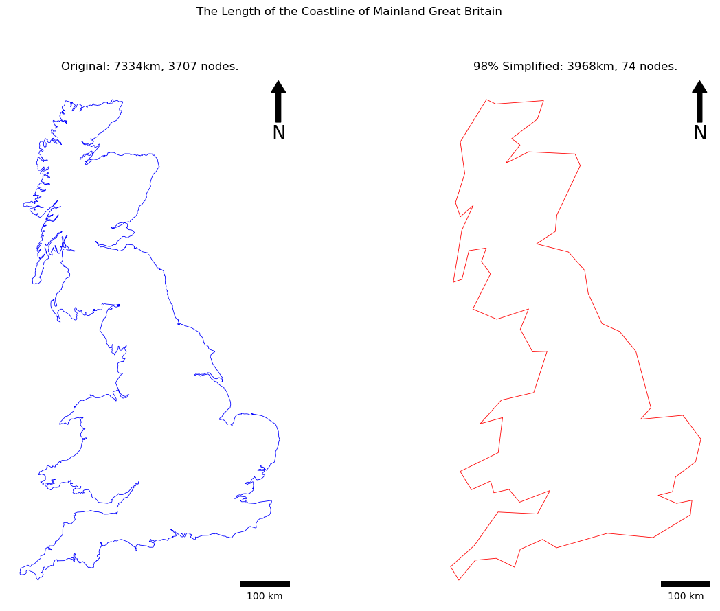
As you can see, this is a highly generalised representation of the coastline of mainland Great Britain!
Though the difference is very obvious here - you might be surprised how much data you can remove before it really becomes noticeable! For example, here is the same data with 80% of the nodes removed:
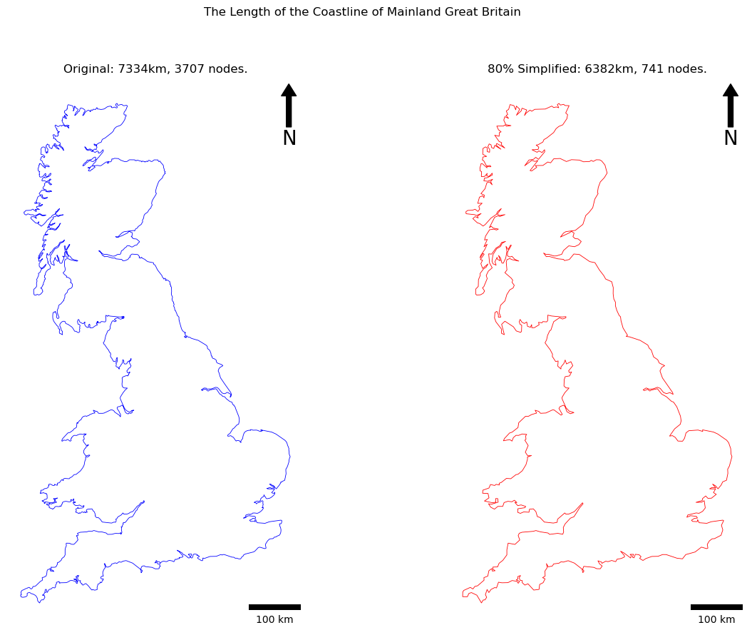
This is of key importance when it comes to communicating data, and obviously has a huge impact on our ability to measure lengths, as two features could look identical to the naked eye, but have huge differences in length (nearly 1,000km in the above example)!
Have a play with your code by editing the
SIMPLIFICATION_PERC- see how good a trade-off you can get between making it appear as a good representation, but still keeping the number of nodes as low as possible.
Once you are happy that you understand it - Congratulations! you now understand generalisation and the Coastline Paradox. Just remember, ALL spatial data are inherently generalised - and it is important that you understand how this will affect your analysis before you start, particularly if you are comparing multiple datasets!
A little more…?
- There is one other loop in this practical that should be converted to list comprehension, find and convert it! (Hint - it is also in the
visvalingam_whyatt()function). - Edit your code so that you undertake this generalisation for all of the polygons in the
MultiPolygon(hint: you will still want to separate theMultiPolygonout into individual polygons!)
The second of these activities is a bit of a challenge, and a great way to build your coding skills! In support of this, consider the following:
To make your output map look good, it would be worth eliminating the smallest islands. I would achieve this using another conditional statement:
# eliminate polygons that are too small
if poly.area > 500000000:
You will likely need to create variables outside of your loop to keep track of the changing lengths, and store a list of your original and simplified LineStrings:
# init counter variables
original_nodes = 0
original_len = 0
simplified_nodes = 0
simplified_len = 0

# init lists to hold the results
original_lines = []
simplified_lines = []
Remember, you can view the solution here and post questions on the forum if you get stuck. If it goes well, you should get something like this:
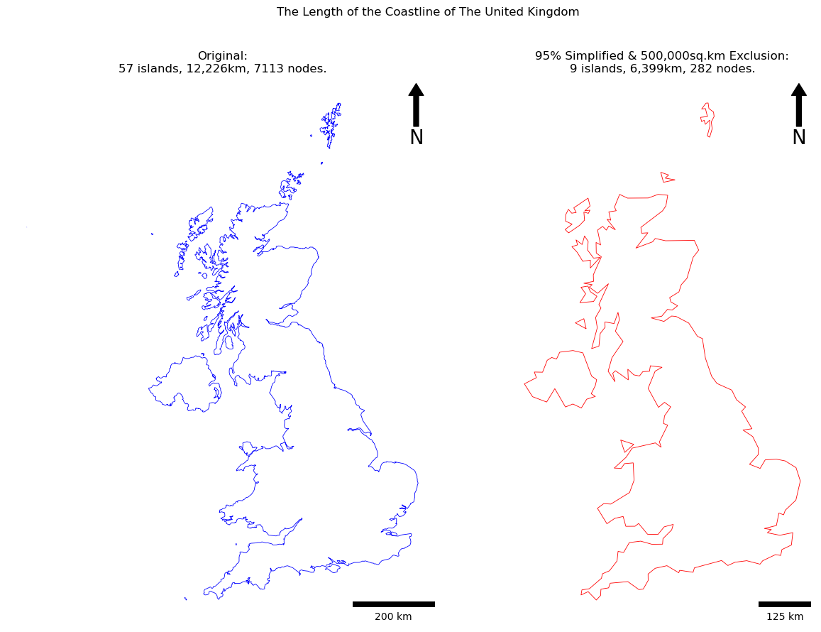
Enjoy!