In which we get to grips with raster data, and reproduce a classic algorithm to model flood extents.

Part 1

Working with Rasters

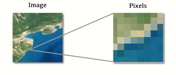
This week we are going to move on from the vector data upon which we have focused so far; and towards the other major data type in GIS: Raster data. As we saw in the lecture - a raster dataset comprises a surface of cells (also known as pixels), just like a digital photograph:

Specifically, we will be using a Digital Elevation Model (DEM). A DEM is a raster surface in which each cell represents an elevation value (as opposed to storing the colours for a photograph, like the above).

Opening Rasters with rasterio

So far, we have been accessing vector data using geopandas and its GeoDataFrame Object, as we have discussed previously, geopandas is quite a high-level library that is really aimed at functional programming applications - though it has worked fine for us in our object-oriented programming approach. We selected this over a lower-level library as it makes it a little easier for us to plot maps (the details of which are not really the core purpose of this course). For raster data we will use a lower-level library called rasterio:

Create a new file called week7.py in your Week 7 directory, and add the below snippet to import the necessary function from rasterio

from rasterio import open as rio_open

Note that I have also used a slightly unusual import statement here, in which I have re-named the open function to rio_open using the as keyword. This is simply because open is a very generic name and I could easily end up adding two libraries that both have a function called open. For this reason, it is often handy to re-name imports as I have done here to avoid confusion!

The traditional way to store raster data is using an ASCII dataset (.asc file) - this is a simple text-based file that looks like this:

ncols 200
nrows 200
xllcorner 330000
yllcorner 510000
cellsize 50
263.9 251 233.6 222.6 210.8 195.9 185 177.4 169.7 167.3 167.8 168 168 168.6 167.9 168.1 170.8 171.4 168.8 168.7 173.6 168.5 173.1 173.4 178 180.6 196.6 205.6 214.7 230.8 252.6 270.7 273.5 264.4 224.3 188.1 158.2 155.9 171.7 193 213.9 234.6 257.4 272.1 295.3 318.8 338.3 358.8 385.8 416.7 434.8 451.6 462 479.8 493 504.1 519.8 531.4 537.7 539.8 549.6 554.8 562.8 574.3 581.4 584.6 591.7 599.3 602.3 613.7 630 646.4 663.9 677.6 693.2 710.2 729.6 746.7 765.5 781.9 788.3 790.9 787.8 781 772.2 758.7 747.1 736.4 725.9 715.6 700 684 668 654.5 642 631 618.2 607.5 598 586.2 574.6 564.6 554.9 548.6 540.9 533.7 530.4 527.8 530.9 535 551 572.2 593.6 616.7 637.3 659.5 675.5 681.1 687.9 691.3 691.8 690.5 689.8 688.5 683.4 671.9 688.4 695.7 699.4 696.1 689.1 678.1 664.4 649.2 633.8 619 600.8 587 573.5 560.3 554.1 544.1 528.7 516.6 509.2 502.9 498.6 493.9 488.9 479.9 485.4 495.4 505.8 517.8 528.1 541.3 538.9 532.7 525.8 519.3 505.4 498.6 492 480.9 470.7 458.4 443.3 426.4 409 384.5 362.9 345.1 326.1 310.5 295 275.7 267.1 256.6 246.5 236.6 228.3 221.4 216.5 212.4 207.3 199.6 194.6 187.6 180.4 174.5 173.6 171.4 169.9 166.8 162.7 164.1 166 165.9 164.3 162.2
287.9 284.9 267.9 247.6 229.1 214.3 197.5 185 175.4 167.4 167.4 168 167.8 168.6 168.8 168.5 168.5 176.7 180.5 168.8 169.2 169.2 180.1 183.9 177.4 175.8 182.9 189.8 201.5 230.8 258.6 264.3 249.7 232.5 194 163.5 157 159.5 178.6 200 219.5 234.8 247.5 267.3 287 311.5 335.3 361.1 386.2 399.5 418.1 431.9 431.1 456.1 465.2 475.5 503.2 509.9 516 540.8 549.2 554 558.8 565 582.7 595 601.5 610.2 621.2 633.7 644.4 662.4 677.6 696.5 715.3 733.3 750.5 765.9 778.8 786.3 787.8 786 779.8 769.3 753.3 739.3 730.3 721.6 711.5 700.3 687.3 671.5 656.9 644.3 632.2 621.1 609.6 602.8 595.7 581.1 570.5 561.4 548.3 543.5 546.1 536.3 530.7 532.9 536.8 549 560.4 581.8 610.3 641.1 670.2 684.4 698 703.4 706.4 708.1 704.4 701.2 698.4 696.1 691.2 689.2 696.6 705.3 709.9 709.1 702.3 692 678 658.6 643.5 629.1 612.9 595.9 583 575.4 566.2 551.3 534.3 521.5 514.9 508.7 502 496.6 491.9 479.9 491.6 499.6 509 521 531.4 539.7 544.5 534.7 524.4 516.8 507.6 499.5 492.9 481 467.9 454.8 438.1 419.1 388.7 366 347 327.9 312.9 297.2 281.9 272.6 262.3 251.1 237.7 229.7 223.1 216 211.5 207.1 201.5 194.9 189.7 183.1 174.5 172 170.6 168.8 167.9 162.3 158.8 158.1 159.2 161 159.5 157.5
303.3 309.6 299.9 276.4 255.1 239.3 220.7 197.4 182.5 170.2 167.4 168 167.8 168.2 167.4 167.8 168.3 168.9 172.3 170.1 170.4 169.3 183 188.8 178.8 183 177.4 181 194.9 224.7 240.3 243.7 225.5 201.4 177.2 157.4 159.1 163.4 185.5 207 228.4 236 248.5 263.3 285.8 313.1 335.3 354 360.7 394.1 397.4 438.2 458.4 475.4 495.4 504.4 496.6 509.7 528.2 550.8 565.1 575.6 585.1 593.1 597.8 608.4 617.8 626.1 636.8 647.9 662.3 677.6 696.1 712.4 734.8 753.5 766.8 776.3 783 784.6 782.5 777.3 768.5 752.3 730.9 715.1 709.1 703.7 695.3 684.2 671.2 658.6 645.3 633.3 622.7 613.3 602.3 598.9 596.4 576.9 567 558.8 555.6 560.2 555 540 533.6 536.8 542.1 558.9 573.9 597.5 628.3 659.7 685.8 705.4 716 722.2 723 721.1 714.5 707.6 705.6 703.6 699.1 698.5 705 710.9 714 714 710.2 701.8 687.7 670.3 652.2 633.1 616.1 602.7 592.2 584.4 570.9 556.6 538.2 525.3 517.9 510.9 504.6 499.7 492.1 488.3 495.8 503.2 512.5 521.1 531.4 538.3 545.2 538.5 528 515.9 511.4 504.7 494.6 479.5 465.2 444.1 428.5 405.2 378 354 335.6 316.3 300.2 286.8 276.9 267.8 260.2 245.8 232.8 224.6 218.5 211.7 206.8 202.5 196.7 191.3 184.7 179.2 173.1 171.3 170.9 172.7 166.9 163.1 161.5 159.9 153.6 154.8 153.4 152.5
...

Check this yourself by opening Helvellyn-50.asc in a Text Editor such as Notepad (Windows) or TextEdit (Mac)

As you can see - the file comprises a series of header lines, which describe the dimensions (ncols, nrows), location (xllcorner, yllcorner), and resolution (cellsize) of the dataset. These header lines are then followed by the data itself (I have included only the first three lines here - but as described in the header there are 200 in the file).

There is at least one clear issue with this format that should be leaping out at you - can you think what it is…?

…hopefully you have identified that the file contains nothing describing a CRS! This is important, as it means that the operator has to know what CRS to use, otherwise the data are useless (we don’t know the units of the coordinates or resolution, and the georeferencing information is meaningless). As with Shapefiles (which are another rather outdated format), ASCII files will tend to pick up a selection of sidecar files (e.g., a .prj file to describe the CRS).

Check this out as well by opening Helvellyn-50.prj in your text editor

For this reason, we would normally prefer to use a more modern format, such as GeoTiff. This is not a format that you can view in a text editor, but it has many benefits over other data formats such as .asc, including being faster to read, much more space-efficient and (crucially) storing the CRS!

It is also noteworthy that, unlike vector data, each data point in this raster dataset is not related to an explicitly defined location (i.e., only the coordinates of one corner are recorded). This means that we have to work out the coordinates for the rest of the cells based on the cell size (resolution) and the distance (measured in cells) from the known corner. Clearly, accidentally skipping or deleting a row, column or cell would therefore have a huge impact on the dataset!

To open a raster dataset (a GeoTiff file in this case), we simply use the rio_open function that we imported. There are two ways to do this:

1. The Traditional way:

# open the file
dem = rio_open('../data/helvellyn/Helvellyn-50.tif')

# do something with it...

# close the file
dem.close()

2. using a with statement

# open a raster file into a variable called dem
with rio_open('../data/helvellyn/Helvellyn-50.tif') as dem:

	# everything inside the with block can access dem
  
# once you leave the block, the file automatically closes for you

As you can see - the approach that uses the with statement is a little easier to use, as it avoids the need to remember to close the file (if you forget this, then it will remain in memory). For this reason, we will use the with statement to open and close raster datasets.

When we are inside the with statement, we have access to the dem variable (which you could call anything that you like as it is a variable). As soon as you leave the with block (the indented bit), the file is safely closed by Python and the dem variable is destroyed.

Make sure that you fully understand how the with statement works with rio_open - if you don’t get it, ask!

Add the above snippet (the one using the with statement) into your code to open the raster data file. Note that the code will not run successfully until you have put something inside the with statement, so don’t test it yet!

rasterio data structures

rasterio has its own data structure. The structure is simple, but you need to make sure that you understand it in order to be able to access the data that you want correctly.

Raster data are organised into bands, which can be thought of like layers. Each band is the same size, and covers the same area, and the cells of each band align perfectly.

A DEM (Digital Elevation Model) like we have here is a simple raster dataset, because it only contains a single band (representing elevation). A satellite image, for example, is a little more complex, because it contains three bands: the first of which contains the red component of the colour for each cell, the second of which contains the green, and the third of which contains the blue (this is exactly the same as normal digital photographs). When we open an image file for viewing on our computer, the software combines the red, green and blue components of each cell to give the final colour that we see on our screen (each pixel of which is made up of three tiny LED’s - one red, one green, one blue…). Some Multispectral datasets like you might see in remote sensing datasets can have many bands.

Let’s have a look at the structure of our dataset:

Add the below snippet and now run your code to test that the dataset has been opened successfully.

print(dem.profile)

This allows you to see lots of information about the raster dataset that you have opened, including:

The CRS in raster data is important, as rasters must be projected (as they are made up of square cells). You can certainly de-project a raster dataset (e.g. to WGS84), but it will be implicitly forced into the equirectangular projection by the GIS. In our case, we are using elevation data from the Ordnance Survey that is already projected to the British National Grid, so there is nothing further for us to do here.

The bands of a raster are ordered in a list, which is accessed using the .read() function, passing in the number of the band in which we are interested (1 in this case) - note that this is the number of the band and not an index value - so it starts at 1 and not 0!

# get the single data band from a dem
band_1 = dem.read(1)

If we didn’t have a DEM, but had an aerial photograph instead (for example…) then we could have three bands to access like this:

# get the rgb components from a photograph (img)
red_band = img.read(1)
green_band = img.read(2)
blue_band = img.read(3)

Alternatively, you can just store all of the bands in a list with read() (no argument), and then extract them as normal:

# get the rgb components from a photograph (img)
bands = img.read()
red_band = bands[0]
green_band = bands[1]
blue_band = bands[2]

Add the necessary line to read the single band from the dataset into a variable called dem_data.

Managing coordinate space

Once you have the band that you want, you need to deal with one of the fundamental issues of raster data: the fact that computers store cells of data referenced using the x,y coordinates from the top left (which we call image space), whereas coordinate reference systems (and so GIS…) store them using x,y coordinates from the bottom left (which we call coordinate space). See here:

Translating projected coordinates (e.g. 345678, 456789) into raster coordinates (e.g. 263, 100) has traditionally been a major source of error for programmers because it is easy to get wrong, but fortunately rasterio makes this very easy for us.

All we have to do is use the .index() and .xy() methods to convert between x,y coordinates in a spatial reference system (coordinate space), and column,row locations in a raster dataset (image space). Under the hood, this is done using the Affine Transformation Matrix that we saw earlier, but these handy functions mean that we no longer have to deal with these directly.

Here is how they work (where d is the dataset - in our code this is called dem):

'''
convert between coords and array position
returns row,col (y,x) as expected by rasterio
'''
row, col = d.index(x, y)

'''
convert between array position and coords
params are row,col (y,x) as expected by rasterio
returns coords at the CENTRE of the cell
'''
x, y = d.xy(row, col)

These functions are brilliant, as they mean that we can move between coordinate space and image space very easily. This saves time, effort and lots of potential errors!

Accessing values from a raster dataset

Now that we can open the dataset and we know how to move between coordinate space and image space, we simply need to know how to read values out of the dataset. Each band is stored in the dataset as a two dimensional list, which can be accessed in the form dem[row][column]. This makes extracting the data very simple:

1. Translate the coordinates for which we would like to extract the data into image space (row and column)
2. Use the row and column indices to read values out of the the two dimensional list (the band)

Here it is:

# transform the coordinates for the summit of Helvellyn into image space
row, col = dem.index(x, y)

# print out the elevation at that location by reading it from the dataset
# note that this makes use of an f-string to format the number
print(f"{dem_data[row][col]:.0f}m")

You can even streamline this a little by passing the results of .index() directly as an index value to dem_data. This works because of a handy feature of numpy arrays that allow you to access data at a given index:

# access data from an array like you would in a list
value = dem_data[row][col]	# this would also work on a list

# access data from an array using a tuple
value = dem_data[(row, col)]	# this would NOT work on a list	

Because .index() returns a tuple in the form (row, column), and the array will understand this as an index position, we can put the function call right into the square brackets and read the result from the dataset in a single line:

# print out the elevation at that location by reading it from the dataset
print(f"{dem_data[dem.index(x, y)]:.0f}m")

We can also use the same trick to write values to specific cells in the raster dataset:

# set the cell at x, y to 1
dem_data[dem.index(x, y)] = 1

Got it? Great, now see if you can put all of that together to complete a little challenge:

Using the above, see if you can find the elevation of the summit of Helvellyn (coordinates: 334170, 515165) - swap out these coordinates for x and y as appropriate in one of the above snippets

If you got it right, you should have something like 941m.

Note that this is slightly different to the value that you will get from Google because of generalisation in the dataset, which is a direct result of the approach taken to convert the continuous shape of the landscape into the discrete cells of the raster. This is analogous to the generalisation in vector datasets that is caused by attempts to convert a continuous shape (e.g. a coastline) into a discrete shape (e.g. a LineString) that we learned about last time - the height of the mountain will vary depending on the dataset used to measure it!

Part 2

Flood Fill Analysis

This week we are going to have a go with a simple ‘classic’ raster analysis algorithm: the Flood Fill. Like many raster-based GIS algorithms, it has its roots in basic computer graphics from the 1980’s and 1990’s (you can still see this exact algorithm to this day in Microsoft Paint if you use the “bucket” tool)!

Here, we will be using the algorithm to establish flooding extent. At this point we should be clear that this is a very simple flooding model, and far too simple for direct use in most hydrological applications (which would need to account for a wide range of factors such as land cover, underlying geology etc). It does, however, provide us with a great example of how to work with raster data (which is what we are really trying to achieve today) and the approach that we use here is nevertheless the basis for many other more complex models.

Specifically, our algorithm will allow us to specify a location in a landscape and a height - and it will identify the extent of contiguous flooding that would be required for the water to be that high at this location (assuming that the ground is completely saturated). Here is an example of the result of a 2m high flood at the location specified by the red dot:

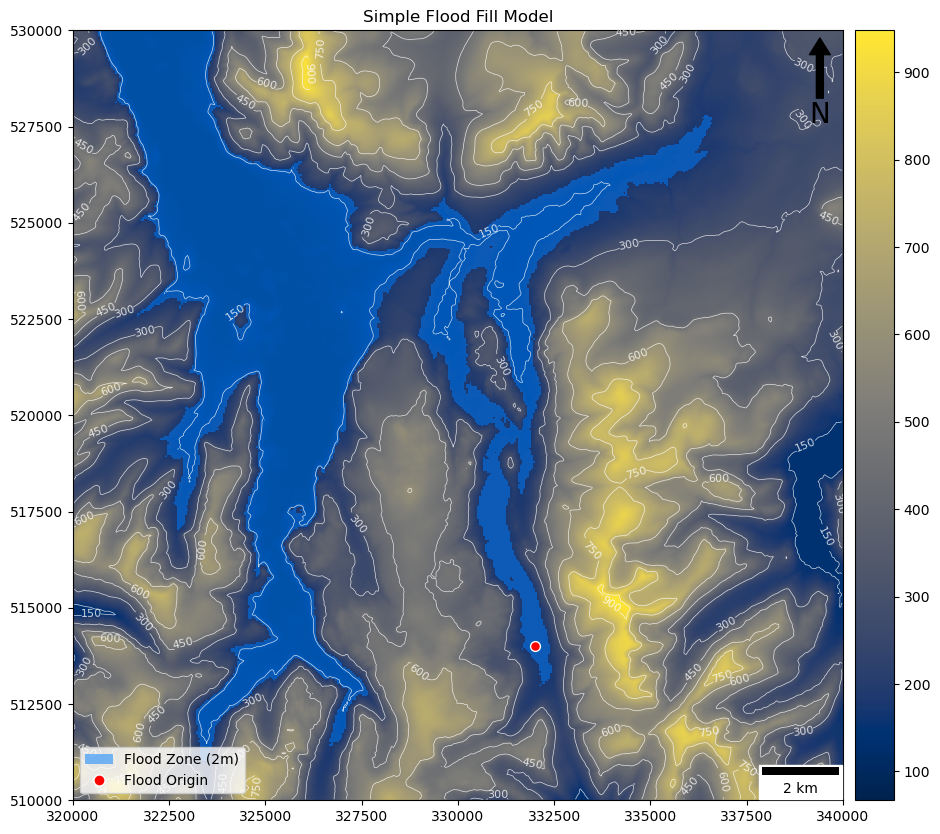
See how that works? Theoretically, we would be able to use this, for example, to predict flooding extents based on sample depths (but once again - the reality of hydrological modelling would be much more complex than this example).

Let’s get started right away:

Replace your existing code from Part 1 with the below snippet:

from rasterio import open as rio_open

# open the raster dataset
with rio_open("../data/helvellyn/Helvellyn-50.tif") as dem:

    # read the data out of band 1 in the dataset
    dem_data = dem.read(1)

Creating Raster Data

In raster analysis, it is usually that case that you will want to output a new raster dataset. Let’s start by taking a look at what we have got, after which we can take a look at how to make a new one:

from rasterio.plot import show as rio_show
from matplotlib.pyplot import subplots, savefig

# plot the dataset
fig, my_ax = subplots(1, 1, figsize=(16, 10))

# add the DEM
rio_show(
  dem_data,
  ax=my_ax,
  transform = dem.transform,
)

# save the resulting map
savefig('./out/6.png', bbox_inches='tight')

Add the above snippets to suitable locations in your code and run it

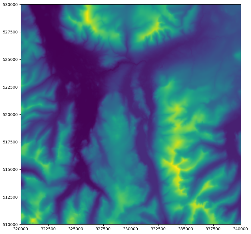
You should get something like this:

That is our base data - it is a DEM of the same area of part of the Lake District.

To create a new raster dataset, we basically need to create a blank surface to draw to - this is effectively a new raster dataset that perfectly matches the dem data that we have already; except all of the values will be 0.

We can create this by using a handy function called zeros(), which is part of the numpy (numeric Python) library that we used last week. This creates a list of 0s (actually, it is a special type of list created by numpy called an array - this is exactly the same thing as rasterio uses to store its data, but for our purposes we can just consider it to be another type of collection like a list). We will pass the dimensions of our existing dataset as the argument to the zeros() function, meaning that we get a 2-dimensional numpy array that is exactly the same size as our existing dataset. This means that we can borrow the CRS and affine transform matrix from our dataset, and they will make it fit perfectly with the map that we already have!

Add the below snippets to your code at the appropriate places to add a layer of 0’s to your dataset. Think carefully about where each snippet should go in your code

from numpy import zeros

# create a new 'band' of raster data the same size
output = zeros(dem_data.shape)

Note that dem_data.shape returns the dimensions of the array as a tuple - it is the equivalent of (dem.height, dem.width) (note that this goes height, width because it is in image space!) - in practice, either would work perfectly fine, but the .shape version is easier to remember and has a lower chance of making a mistake!

Now we have our array of 0’s, we can take a look at it by plotting it on top of our DEM using the affine transform object from the DEM (dem.transform):

# add the empty layer
rio_show(
    output,
    ax=my_ax,
    transform=dem.transform
    )

Add the above snippet to the appropriate location in your code and run it

If all has gone to plan, you should now have something like this:

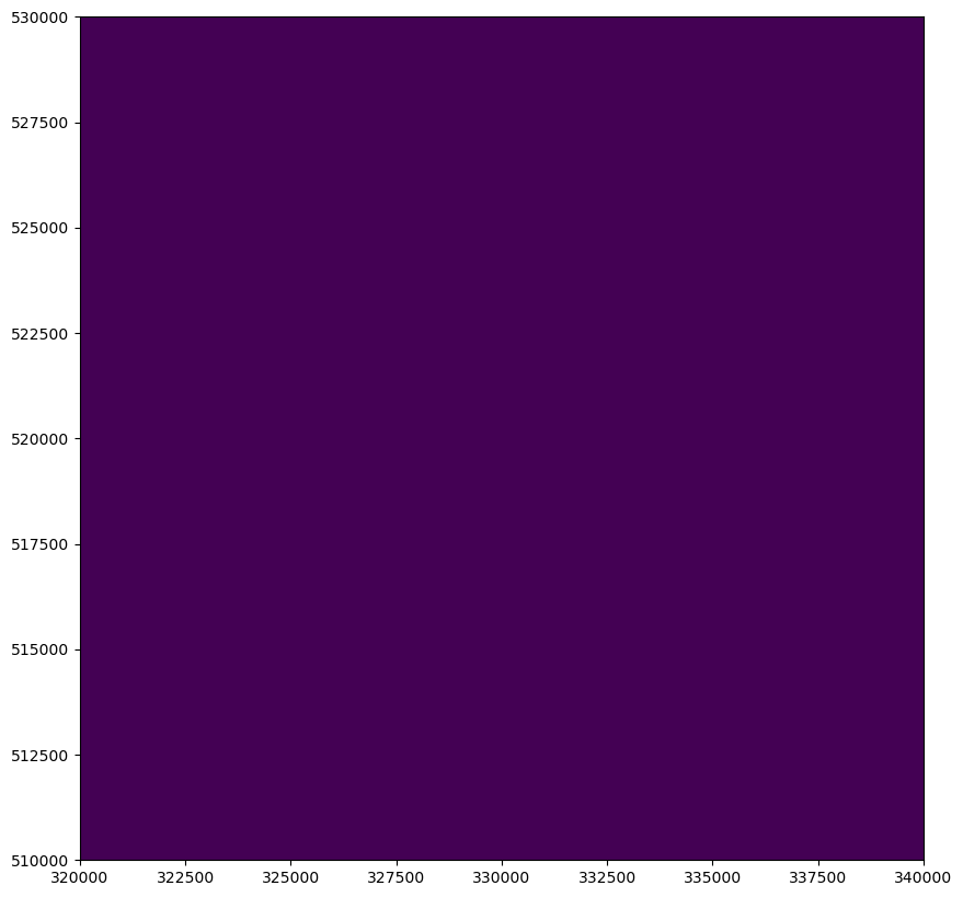
This is what we are expecting, because we have added a layer over the top of our DEM that has all 0s!

Next, we want to edit the colour map of this layer, so that it does not obscure our DEM. We are going to do this using a classified colour scheme, in which we have two possible values:

• 0: invisible, areas that we have not drawn on
• 1: blue, areas that we have drawn on

We achieve this by adding a list of tuples comprising four values, each of which is a number on a scale of 0-1. In order, they represent:

1. Red (how much red is in the resulting colour)
2. Green (how much green is in the resulting colour)
3. Blue (how much blue is in the resulting colour)
4. Alpha (the opacity of the resulting colour - where 0 is transparent and 1 is opaque)

To apply this approach, add the following snippet to your code at the appropriate location…

from matplotlib.colors import LinearSegmentedColormap

… then add the following snippet as an additional argument to be added to the rio_show(output, ...) function call that draws the empty layer:

cmap = LinearSegmentedColormap.from_list('binary', [(0, 0, 0, 0), (0, 0.5, 1, 0.5)], N=2)

Here, we are using a the .from_list() function of the LinearSegmentedColormap object from matplotlib. This is used to create a new LinearSegmentedColormap - which simply means a ‘standard’ colormap where values are related to two or more colours. As you would expect, .from_list() is simply used to create the LinearSegmentedColormap from a list of colours (represented as tuples of 4 values, as described above). We define how many colours using the N argument, provide the list as the second argument, and give our new colormap a name ('binary' in this case) with the first argument.

As you can see, our colour scheme has two colours (N=2):

• 0: transparent black (0, 0, 0, 0)
• 1: semi-opaque blue (0, 0.5, 1, 0.5)

This means that values in the raster that =1 will be shown as blue, and values that =0 will be transparent. From a programmers perspective, a LinearSegmentedColormap object is basically just a function - you pass a collection of values (0 or 1) and it returns a list of the appropriate colours - rio_plot() uses this to colour each individual cell in the raster dataset when we plot it onto a map.

Make sure that you understand the above (if not, ask!) and then run your code

If all goes to plan, you should now have returned to your original image (because the new image is all 0s, and so completely transparent):

Drawing to your new Raster Layer

Now we have a transparent layer laying perfectly over our map, and we know that any cells that we set to 1 will appear as blue (as per the colour map above).

Lets start by editing one cell - we will mark the summit of Helvellyn (the highest and therefore most yellow mountain in the area) with a blue point.

We know the coordinates of Helvellyn from Part 1 (334170, 515165). All that we therefore need to do is convert these coordinates to Image Space, and then set the corresponding cell to = 1!

Set the value in the array position that corresponds to the location (334170, 515165) as 1 and re-run your code (we saw how to do this in Part 1)

If all went to plan, you should see the summit of Helvellyn go blue (you need to look closely, it is only a change of one cell! Note that you can use the coordinates on the axes to help you find it…):

Setting a Suitable Colormap

The default colormap (so called because it maps colours to values) shown above is a very good one (which is why it is our default), but it might not work well with our application today because we are going to draw flood water in blue; and so we ideally want to use one that is a little less blue to avoid confusion!

Take a look at the colour map information on the matplotlib website here

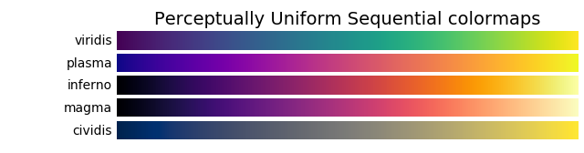
As you can see, the default is the viridis colormap from the perceptually uniform sequential colormaps collection - this means that equal steps in data are perceived as equal steps in the color space. For many applications, a perceptually uniform colormap is therefore the best choice. You can read more about selecting appropriate colormaps for various applications here, and there is a well-known tool that suggests suitable colormaps for various purposes here. There is also an excellent article called The misuse of colour in scientific communication that is well worth a read! The below image is from that article and illustrates the issue very nicely:

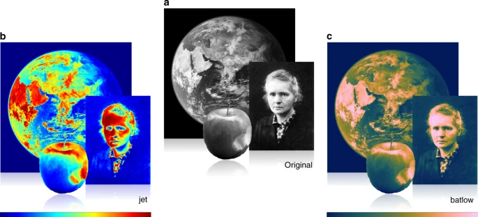
Source: Crameri et al. (2020).

Four such options are available to us in pyplot:

Set a new colour ramp from the above by adding a cmap argument to the rio_show() function. This should be set to a string containing the name of your chosen colour ramp (e.g., to keep the same one you could add cmap='viridis')

The Flood Fill Algorithm

Now that we have got the hang of this, you can save and close this file. Create a new file called week7/7_flood.py and put the code from the below snippet into it:

from numpy import zeros
from rasterio import open as rio_open
from rasterio.plot import show as rio_show
from matplotlib.pyplot import subplots, savefig
from matplotlib.colors import LinearSegmentedColormap

# open the raster dataset
with rio_open("../data/helvellyn/Helvellyn-50.tif") as dem:  # 50m resolution

    # read the data out of band 1 in the dataset
    dem_data = dem.read(1)

Now that we know how to create an output layer and make it turn blue, we simply need to work out which ones we want to flood! For this we will create a function called flood_fill():

Add the below snippet to your code:

  # calculate the flood
  output = flood_fill(FLOOD_DEPTH, LOCATION[0], LOCATION[1], dem, dem_data)

Add the missing flood_fill() function definition to your code - call the arguments depth, x0, y0, d and dem_data), and remember that functions should be located at the top of your code, below the import statements!

Note that we are passing the dem object (rasterio dataset) and the dem_data (array containing the data from band 1 of dem) - this is just for efficiency (to avoid having to call dem.read() a second time). Both are required, because we need the DEM data, but also the .index() function (which is a function of dem).

Add the below snippet to your flood_fill() function to create the output dataset that we will populate with our flooded area:

  # create a new dataset of 0's
  flood_layer = zeros(dem_data.shape)

As you saw in class, the flood fill algorithm is simply a matter of:

1. starting at a given cell and flooding it…

2. checking if each neighbour cell will therefore flood, and flooding it as appropriate…

3. checking if each neighbour of each of the flooded neighbours will therefore flood, and flooding it…

4. …and so on… until you run out of neighbours (i.e., you don’t flood any new cells)

Simple!

Let’s start by defining our settings:

Add the below snippet at the appropriate location (not inside the flood_fill() function!)

# set the depth of the flood
FLOOD_DEPTH = 2

# set origin for the flood as a tuple
LOCATION = (332000, 514000)

Note that we have defined these variables in SNAKE_CASE in upper case, rather than in lower case like usual - this is a common convention when we add settings to our code (i.e., variables that a user might edit to use our script). This doesn’t affect the running of the code, it is simply a convention to help keep your code clear!

The first thing that we want to do in our flood_fill() function is to convert the origin of the flood (x0, y0) from coordinate space (x,y) to image space (row, column).

Add and complete the below statement to your function to achieve this, noting how we are using variable expansion to store the results in two variables: r0 and c0.

	# convert from coordinate space to image space
  r0, c0 = 

Next, we will initialise two collections to help us keep track of which cells have already been assessed (to avoid us continually re-checking the same cells), and which should be assessed in the next iteration of the algorithm. Here we will choose sets, which are like a list, but with the distinction that they do not accept duplicates. This is very useful to us here, as we do not want to be assessing cells more than once (which would be inefficient) - so the alternative would be constantly checking whether a value is already in the collection before we put it in. This way, we can just add all items safe in the knowledge that any duplicates will be quietly rejected!

  # set for cells already assessed
  assessed = set()

  # set for cells to be assessed
  to_assess = set()

Add the above snippet to your code

To get the ball rolling, let’s add our current cell to the list of those must be assessed

Add the below snippet to your code

	# start with the origin cell
	to_assess.add((r0, c0))

Finally, we need to work out the elevation of the flood (which is the sum of the elevation of the origin cell and the depth of the flood).

  # calculate the maximum elevation of the flood
  flood_extent = 

Add and complete the above snippet to achieve this (check the arguments of your function if you need a clue)

Take a look at your function at this point and make sure that you understand it

The ‘Main Loop’

We are now ready to start the ‘main loop’ of the function. As you saw in the lecture, we will now continually iterate through the to_assess set until it runs out. At each step, we:

1. Assess whether the current cell should flood (based on its elevation)

2. If so, set it to 1 in the output dataset and add all of its neighbours to the to_assess set

3. If there are any more cells in the to_assess set, get the next one and go around again…

As with the Visvalingam-Whyatt algorithm that we looked at last time, this kind of situation is perfect for a while loop:

	# keep looping as long as there are cells left to be checked
	while to_assess:

Note that we do not need to write while len(to_assess) > 1 as you might be expecting - this would work too, but for convenience Python evaluates an empty collection to False.

Our first step in the loop is to move the current cell from the to_assess set to the assessed set - this is important as it means that it will not be assessed again in the future!

    # get the next cell to be assessed (removing it from the to_assess set)
    r, c = to_assess.pop()

    # add it to the register of those already assessed
    assessed.add((r, c))

Note that, as with a list, .pop() removes and returns the first item in a collection. The .add() function of the set object is similar to the .append() function of the list object.

Make sure that you understand this, then add the above snippets to your code

Next, we need to decide whether or not the current cell (defined by (r,c)) is going to flood and if so, set the value in the output dataset (flood_layer) to 1.

Add two lines of code to achieve this

Getting to know your neighbours

Now we have updated the value for this cell, we need to add its neighbours to the to_assess set. The neighbours are the 8 cells that surround it. Here is one way to achieve this:

# compile a list of valid neighbours
neighbours = []										
neighbours.append((r, c-1))			# up
neighbours.append((r, c+1))			# down
neighbours.append((r-1, c))			# left
neighbours.append((r+1, c))			# right
neighbours.append((r-1, c-1))		# top left
neighbours.append((r+1, c+1))		# bottom right
neighbours.append((r-1, c+1))		# bottom left
neighbours.append((r+1, c-1))		# top right

Make sure that you understand this, bearing in mind that it uses image space, so the + and - on the y axis are the opposite to how they would be in coordinate space.

One issue that you must always be aware of when dealing with raster cells is that you have to be careful not to ‘fall off’ the edge of the dataset. For example, if you were assessing a cell on the top row of the raster and tried to assess one above it, you would get an Index Error. Such errors are inevitable in an algorithm like this one, so we must control for it. One approach to this would be the below:

# compile a list of valid neighbours
neighbours = []
if c > 0:												# up
    neighbours.append((r, c-1))
if c < d.height-1:									# down
    neighbours.append((r, c+1))
if r > 0:												# left
    neighbours.append((r-1, c))
if r < d.width-1:									# right
    neighbours.append((r+1, c))
if r > 0 and c > 0:								# top left
    neighbours.append((r-1, c-1))
if c < d.height-1 and r < d.width-1:		# bottom right
    neighbours.append((r+1, c+1))
if c < d.height-1 and r > 0:					# bottom left
    neighbours.append((r-1, c+1))
if c > 0 and r <  d.width-1:					# top right
    neighbours.append((r+1, c-1))

Make sure that you understand how this prevents you from selecting any cells beyond the extent of the dataset

Whilst perfectly valid, an approach like this is not very elegant - it perhaps a little long-winded, and results in a list of neighbours that we would subsequently have to loop through in order to check if we had assessed them, and (if not) add them to the to_assessed set:

# loop through each neighbour
for neighbour in neighbours:
  
	# ...if they have not been assessed before
	if neighbour not in assessed:

		# ...then add to the set for assessment
    	to_assess.add(neighbour)

This is an example of a situation in which you are creating a list then immediately looping through it. In such situations (assuming that you do not need to use the list elsewhere), it is almost always better to simply combine the two operations into a single loop - this would generally be considered to be a much more elegant approach (which is one of the things we are looking for in the Assessment…).

An example of combining the above two snippets into one would be something like this:

            # loop through all neighbouring cells
            for r_adj, c_adj in [(-1, -1), (-1, 0), (-1, 1), (0, -1), (0, 1), (1, -1), (1, 0), (1, 1)]:

                # get current neighbour
                neighbour = (r + r_adj, c + c_adj)

                # make sure that the location is wihin the bounds of the dataset
                if 0 <= neighbour[0] < dem.height and 0 <= neighbour[1] < dem.width and neighbour not in assessed:

                        # ...then add to the set for assessment
                        to_assess.add(neighbour)

Here we are:

1. using a loop through a pre-defined list of values to describe the position of each neighbour relative to a given cell (this is fine as they are always the same!)
2. using these values, calculate the location of the current cell in Image Space

3. making sure that:

   1. the calculated location is within the bounds of the dataset
   2. the neighbour cell has not already been assessed
4. if so, addding the neighbour to the to_assess set

Note how the three checks that we are doing in step 3 are done using a single if statement, with each check joined with the keyword and. The only bit here that might be a bit unfamiliar here is the use of the between comparison syntax in Python (0 <= neighbour[0] < dem.height and 0 <= neighbour[1] < dem.width). This is simply a shorthand that allows you to turn a conditional statement like this:

# check if a number is between 0 and 10
if number >= 0 and number <= 10:

to this:

# check if a number is between 0 and 10
if 0 <= number <= 10:

Can you see how that works? There is no benefit to this other than it is a little shorter and neater. Note how we flip the ‘greater then or equal to’ operator (>=) to ‘less then or equal to’ (<=) to reflect the change in order of the values.

Make sure that you understand how this achieves the same things as the two snippets above it

Add the above snippet (the ‘elegant’ version using the between statement) to your code

Finally, we simply need to return our resulting flood layer from the function:

Add the below snippet to complete your flood_fill() function

  # when complete, return the result
  return flood_layer

At this point we should have a perfectly functional flood_fill() function!

Let’s add a statement to our main body of code (not the function!) to give it a quick test:

print(output.sum())

This will use the .sum() function of the array object add up all of the values in your output array. Given that you know all of the values are either 1 or 0; a value >0 will suggest that the code is working fine.

Add the above snippet to your code at the appropriate location (after the function call) to see if it is working

If all has gone to plan, you should have a number like 29379.0, meaning that 29,379 (of 160,000) cells in your dataset will be flooded.

Plotting your map

Finally, all that remains is to make it into a map. As we saw above, just like geopandas, rasterio has a built-in plotting function called show(). As with rio_open(), you will notice that we have renamed this function to rio_show() to avoid any potential confusion.

from math import floor, ceil
from geopandas import GeoSeries
from shapely.geometry import Point
from matplotlib.lines import Line2D
from matplotlib.patches import Patch
from matplotlib.colors import Normalize
from matplotlib.cm import ScalarMappable
from matplotlib_scalebar.scalebar import ScaleBar

# output image
fig, my_ax = subplots(1, 1, figsize=(16, 10))
my_ax.set_title("Simple Flood Fill Model")

# draw dem
rio_show(
    dem_data,
    ax=my_ax,
    transform = dem.transform,
    cmap = 'cividis',
    )

# draw dem as contours
rio_show(
    dem_data,
    ax=my_ax,
    contour=True,
    transform = dem.transform,
    colors = ['white'],
    linewidths = [0.5],
    )

# add flooding
rio_show(
    output,
    ax=my_ax,
    transform=dem.transform,
    cmap = LinearSegmentedColormap.from_list('binary', [(0, 0, 0, 0), (0, 0.5, 1, 0.5)], N=2)
    )

# add origin point
GeoSeries(Point(LOCATION)).plot(
    ax = my_ax,
    markersize = 50,
    color = 'red',
    edgecolor = 'white'
    )

# add a colour bar
fig.colorbar(ScalarMappable(norm=Normalize(vmin=floor(dem_data.min()), vmax=ceil(dem_data.max())), cmap='cividis'), ax=my_ax, pad=0.01)

# add north arrow
x, y, arrow_length = 0.97, 0.99, 0.1
my_ax.annotate('N', xy=(x, y), xytext=(x, y-arrow_length),
    arrowprops=dict(facecolor='black', width=5, headwidth=15),
    ha='center', va='center', fontsize=20, xycoords=my_ax.transAxes)

# add scalebar
my_ax.add_artist(ScaleBar(dx=1, units="m", location="lower right"))

# add legend for point
my_ax.legend(
    handles=[
        Patch(facecolor=(0, 0.5, 1, 0.5), edgecolor=None, label=f'Flood Zone ({FLOOD_DEPTH}m)'),
        Line2D([0], [0], marker='o', color=(1,1,1,0), label='Flood Origin', markerfacecolor='red', markersize=8)
    ], loc='lower left')

# save the result
savefig('./out/6.png', bbox_inches='tight')
print("done!")

The only thing different to usual in here is the rather self-explanatory use of rio_show() instead of .plot(), the use of the transform argument (which simply georeferences the raster data), and the use of the cmap (colour map) argument to colour the raster layer. Also note the manual creation of the legend with a Patch (for flooded area) and a point (for the origin point, which confusingly we have created using a Line2D).

Add the above snippets to your code at the suitable locations (remember that some import statements can be merged with existing import statements)

If all has gone to plan, you should get something like this:

A little bit more…?

Try to adapt your code so that it can accept multiple points and depths and work out the worst case flooding zone based on that data.