2. Understanding Topology
A quick note about the practicals...
Remember that coding should be done in Spyder using the understandinggis virtual environment. If you want to install the environment on your own computer, you can do so using the instructions here.
You do not have to run every bit of code in this document. Read through it, and have a go where you feel it would help your understanding. If I explicitly want you to do something, I will write an instruction that looks like this:
This is an instruction.
Remember that we are no longer using Git CMD. You should now use GitHub Desktop for version control.
Don't forget to set your Working Directory to the current week in Spyder!
Shortcuts: Part 1 Part 2
In which we expand our skills in Python, get to grips with topology and geodesy, and start to discover why building Donald Trump’s wall won’t be quite as easy as he thinks…
Getting Ready
Before we start this week, we need to get prepared:
Open up GitHub Desktop and make sure you are logged in and tracking your repository (instructions here)
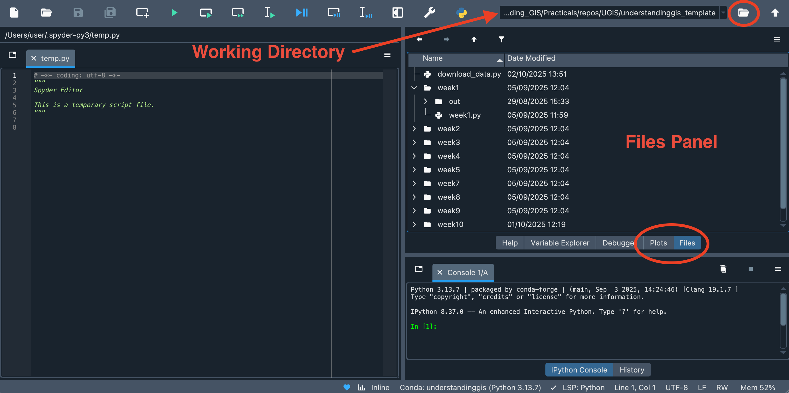
Open Spyder (understandinggis) and make sure that the Working Directory is set to your
understandinggisdirectory. If not, make it so by double clicking on it in the Files Pane or navigating to it using the browse () button in the top right hand corner:
Part 1
Operators in Python
You’ve already seen a few of these in the past week, but an operator is a mathematical symbol that represents an operation undertaken on one or more values or variables (known as operands). In the following table you can see some of the most common operators, along with some examples:
| Operator | Explanation | Symbol(s) | Example |
|---|---|---|---|
| add / concatenate | Used to add two numbers together, OR concatenate two strings together. |
+ |
6 + 9 (15) "Hello " + "world!" (Hello World) |
| arithmetic | These do what you’d expect them to do in basic maths. | -, *, / |
9 - 3 (6) |
| power | Can be used to calculate a number to the power of another number. | ** |
3 ** 2 (9) |
| assignment operator | You’ve seen this already, it assigns a value to a variable. They can also be combined with the arithmetic operators to add a number to the existing value. Note how combining them with an arithmetic operator will perform the operation on the value already stored in the variable, and then store the result back into the variable. |
=+=, -= etc. |
my_var= 7;my_var+= 1 |
| equality operator | This compares two operands, returning True if they are the same, and False if not. |
== |
my_var == 7; |
It helps to be aware of these, though you will quickly get used to them as you write more and more code throughout the course!
Loops and Lists in Python
Lists
Before we get stuck into this week, we are going to learn about Loops and Lists in Python.
The list is one of the most versatile datatypes available in Python - it allows you to store multiple values of multiple different types in a single variable. It is written as a list of comma-separated values (items) between square brackets (e.g. ["one", 2, "iii", fish, "potato"]). One of the best things about a list is that items in a list do not need to be of the same type (as you can see in the example, which is comprised of strings, numbers and variables). This level of flexibility is not available by default in many lower level languages, but it comes at a price in memory usage and speed.
Can you see which are strings, variables and numbers in the above example? If you aren’t sure, ask!
Values stored in a list can be referenced by their index, which is a number describing their position in the list. The index is 0 for the first value, and then increases by 1 for each subsequent value. Values are accessed using their index by using square brackets to indicate which value you are referring to, e.g.:
my_list = ["I", "love", "understanding"]

print(my_list[1])
which gives:
love
Simple!
If you want to add something to a list, then you can do so using the built-in append() function:
my_list = ["I", "love", "understanding"]

my_list.append("GIS")

print(my_list)
which gives:
["I", "love", "understanding", "GIS"]
There are more functions for working with lists in Python, including len(list) to get the number of items in the list, list.insert() to add an item at a specific place in the list, or list.reverse() to reverse the order of the items in the list. You can read more about these methods (and many others) here.
I will often refer you to the documentation for Python and the libraries that we are using - this is important as you need to get used to using them by the end of the course! If you struggle to understand them, just ask!
Loops
One of the main uses for lists is to loop (or iterate) through them, and the most common way to do that in Python is using a for loop.
In simple terms, for statements in Python are a way of making a certain block of code run for every item in a list. To do this, it iterates (moves one item at a time) along the items in the list in the order that it is provided, and then runs a block of code that can access each member of the list in turn. This saves a lot of coding time in comparison to writing everything out multiple times!
Let’s have a simple example:
# create a variable that holds a list of three words
words = ['First', 'Second', 'Third']

# print each of those words in turn
for word in words:
	# everything in the indented block is run for each of the 3 elements in the list
	print(word)
This will print:
 First
 Second
 Third
Open
week2/week2.pyin Spyder and give the above a go, does it work?
Pretty good eh? This is much quicker and simpler than writing out a separate print statement for every word, especially if you have lots and lots of items in the list, or if you don’t know how long the list is going to be ahead of time (which is a common situation in programming).
Let’s have a closer look at the anatomy of a loop:
- The
forkeyword announces to the Python Interpreter that it should expect a loop definition - the
x in ystatement then defines the name of your loop variable (x, orword) in these examples, and the collection (e.g., list -yorwords) that we want to loop through - the colon (
:) then tells the Python Interpreter to expect a block of code. This code will be indented from theforstatement, and will run once for each member ofy- the variable is only accessible from within the code block.
A common variation on this is where you want to do something a certain number of times, but do not have a list upon which to base your loop. The simple way around this is to create a list to give it, which you can do with the range() function. range() simply creates a list of consecutive numbers, starting at 0, that is the length that you request with an argument (arguments** are the values that you put between the brackets in a Python **function). For example:
print(list(range(10)))
gives:
[0, 1, 2, 3, 4, 5, 6, 7, 8, 9]
Give it a go, does it work? Why does it not give 0-10? If you can’t see why, ask!
To use range() in a for loop is very easy, simply:
# loop through a list 0-2
for i in range(3):
     print(i)
which gives:
0
1
2
Once again, give it a go, does it work?
You will notice that, this time, the loop variable (i) refers to the member of the list that range() returns (a number), and not to the corresponding member of words. If you want the member of words you need to access it using words[i] - the square brackets are used to denote which member of the list (based on the index) you are referring to.
for i in range(3):
     print(i, words[i])
NB: I have used i here because it is a convenient letter that keeps the code readable (it is short for iterator). i is just a variable the same as any other, so you can call it whatever you want!
Note that if you pass an index value that is too large, then you will get an error message like this: IndexError: list index out of range . You can, however, pass negative index value, which will count the position from the end of the list instead of the start.
Right let’s have a go:
Use a loop to add all of the below numbers together. I have started you off with some code, paste it in to your file and complete the missing parts to find the solution:
# here is your list of numbers
numbers = [1,2,3,4,5,6,7,8,9,10,15,30]

# this variable will hold your result, start it at 0
total = 0

# MISSING LINE HERE
# loop through the list

	# INCOMPLETE LINE HERE
	# add each number to the total
	total +=

# print the result
print(total)
The answer will be revealed at the beginning of the second lecture segment… Did you get it right?
Finally…

Remember that you do this using GitHub Desktop - not Git CMD!
Part 2
Building Trump’s Wall
Right, now we have got the hang of lists and loops, it is time to put that knowledge to some good use. This week we are going have a look at two major GIS concepts: topology and geodesy.
In his first election campaign (and then throughout his first term), US President Donald Trump talked a great deal about building an ‘impenetrable… southern border wall’ between the USA and Mexico. But exactly how long would this wall need to be? We are going to apply some topology and geodesy to find out…
Filtering your data with geopandas
Right, down to business - we need to calculate the border between the USA and Mexico. Our first job is to identify which geometries in our Shapefile of countries refer to the USA and Mexico, which fortunately is quite simple!
First things first, we need to load in a dataset of countries:
Make a new Python file in your
week2directory and run the below snippet to open a Shapefile
from geopandas import read_file, GeoSeries

# load the shapefile of countries - this gives a table of 12 columns and 246 rows (one per country)
world = read_file("../../data/natural-earth/ne_10m_admin_0_countries.shp")
As we saw last week, the read_file function in geopandas opens a Shapefile and gives us access to the contents through an object which is stored in a variable (in our case, we have called this variable world, but you could of course call it whatever you like!).
This object is a GeoDataFrame, which is the type of object that geopandas uses to hold the tabular data (the attributes) and geometry (the shapes) of this dataset. You can think of a GeoDataFrame as a table, in which each row represents one feature (a country in this case), and each column represents a different attribute of that feature (name, population, GDP etc…) - just like the attribute table in a desktop GIS. Unless you have made some edits, the last column in a geodataframe is always the geometry, which represents the shape of the feature.
As we saw last week, if we just want a simple list of the available columns, you can use world.columns:
Add the below snippet to your code and run it:
# print a list of all of the columns in the shapefile
print(world.columns)
If all goes to plan, you should get something like this, showing 95 columns of data:
Index(['featurecla', 'scalerank', 'LABELRANK', 'SOVEREIGNT', 'SOV_A3',
       'ADM0_DIF', 'LEVEL', 'TYPE', 'ADMIN', 'ADM0_A3', 'GEOU_DIF', 'GEOUNIT',
       'GU_A3', 'SU_DIF', 'SUBUNIT', 'SU_A3', 'BRK_DIFF', 'NAME', 'NAME_LONG',
       'BRK_A3', 'BRK_NAME', 'BRK_GROUP', 'ABBREV', 'POSTAL', 'FORMAL_EN',
       'FORMAL_FR', 'NAME_CIAWF', 'NOTE_ADM0', 'NOTE_BRK', 'NAME_SORT',
       'NAME_ALT', 'MAPCOLOR7', 'MAPCOLOR8', 'MAPCOLOR9', 'MAPCOLOR13',
       'POP_EST', 'POP_RANK', 'GDP_MD_EST', 'POP_YEAR', 'LASTCENSUS',
       'GDP_YEAR', 'ECONOMY', 'INCOME_GRP', 'WIKIPEDIA', 'FIPS_10_', 'ISO_A2',
       'ISO_A3', 'ISO_A3_EH', 'ISO_N3', 'UN_A3', 'WB_A2', 'WB_A3', 'WOE_ID',
       'WOE_ID_EH', 'WOE_NOTE', 'ADM0_A3_IS', 'ADM0_A3_US', 'ADM0_A3_UN',
       'ADM0_A3_WB', 'CONTINENT', 'REGION_UN', 'SUBREGION', 'REGION_WB',
       'NAME_LEN', 'LONG_LEN', 'ABBREV_LEN', 'TINY', 'HOMEPART', 'MIN_ZOOM',
       'MIN_LABEL', 'MAX_LABEL', 'NE_ID', 'WIKIDATAID', 'NAME_AR', 'NAME_BN',
       'NAME_DE', 'NAME_EN', 'NAME_ES', 'NAME_FR', 'NAME_EL', 'NAME_HI',
       'NAME_HU', 'NAME_ID', 'NAME_IT', 'NAME_JA', 'NAME_KO', 'NAME_NL',
       'NAME_PL', 'NAME_PT', 'NAME_RU', 'NAME_SV', 'NAME_TR', 'NAME_VI',
       'NAME_ZH', 'geometry'],
      dtype='object')
A quick look at the column names will give us a pretty good idea of what is in them, and we can be pretty sure that columns like NAME would be a safe bet for identifying which row of data is Mexico, for example. However, the NAME of a country might vary slightly from dataset to dataset (e.g. United States of America, United States or USA might all be valid names). To make our code a little more robust and remove some of the uncertainty, therefore, we will use one of the other columns: ISO_A3. This column refers to the uniqe 3-letter code assigned to each country by the International Standards Organisation. We can say with some certainty that this will be exactly the same in any dataset (as this is the point of a standard!). Looking at the web link clearly shows us that USA has the code USA and Mexico has the code MEX.
We can use this information to extract the relevant countries from our dataset using the functionality of GeoDataFrames to give us advanced data handling techniques. In the case of USA, for example, we simply want to extract the geometry data from the world dataset where ISO_A3 is equal to 'USA'.
We will do that in three steps, and at each step we will print out what class of object we end up with (using the Python type() function), in order to help illustrate how the process works. In object oriented programming, we call the ‘type’ of an object its ‘class’ (a ‘GeoDataFrame object’ is an object of the class GeoDataFrame). Strictly speaking, the class is the code that defines an object - we will be creating some classes later in the course. Here are the three steps:
- From the
worldGeoDataFrame(255 rows x 95 columns), we use the.locproperty of theGeoDataFrameobject to extract a newGeoDataFrame(1 row x 95 columns) containing only the country for which theISO3code isUSA..locexposes the underlying data in a way that allows you to select rows from it using a query. In this case, we seek to extract all of the rows for which our query (world.ISO3 == 'USA') isTrue. The query means: return all of the rows fromworldwhere the value of theISO3column is equal to'USA'). Note how the equality operator is==and not=- this is important to remember -=is the assignment operator (which we use to assign values to variables).
# extract the country rows as a GeoDataFrame object with 1 row
usa = world.loc[(world.ISO_A3 == 'USA')]

print(type(usa))
- From the new
geodataframe(1 row x 95 columns), we use.geometryto extract thegeometrycolumn as aGeoSeries(1 row x 1 column). AGeoSeriesobject ingeopandasrepresents a column of geometry features without any attribute data attached to it. AGeoDataFrameobject therefore effectively comprises aGeoseriesplus a table of attributes.
# extract the geometry columns as a GeoSeries object
usa_col = usa.geometry

print(type(usa_col))
- From the
GeoSeries(1 row) , extract the value from that one row using the.ilocproperty.ilocmeans index location, and is another property of theGeoDataFrameobject, which exposes the underlying data in a way that allows you to select it using a number to represent the row ID (where0is the first row,1is the second, and so on). This is just like with a list (the first member is0) - and in this case we are extracting the first (and only) row. This returns the underlying geometry, which is represented by aMultiPolygonobject from theshapelylibrary.
# extract the geometry objects themselves from the GeoSeries
usa_geom = usa_col.iloc[0]

print(type(usa_geom))
Here we use the the .loc (location) property of the GeoDataFrame object .
Add each of the above three statements to your code one by run and run your code at each step.
If all has gone to plan, you should see your three object types listed as:
<class 'geopandas.geodataframe.GeoDataFrame'>
<class 'geopandas.geoseries.GeoSeries'>
<class 'shapely.geometry.multipolygon.MultiPolygon'>
Can you see what this is showing you? If it doesn’t make sense, ask!
Now, add the missing lines to do repeat the same process for Mexico (
MEX)
Topological Operations with GeoPandas
As we discussed in the lecture, geopandas has lots of built in functions for topological relationships and operations, here is a list of some of the main ones:
| Name | Syntax | Description |
|---|---|---|
| Contains | a.contains(b) |
Returns True or False for whether or not a completely contains b. |
| Crosses | a.crosses(b) |
Returns True or False for whether or not a crosses b. |
| Equals | a.equals(b) |
Returns True or False for whether or not a is exactly the same as b. |
| Intersects | a.intersects(b) |
Returns True or False for whether or not a intersects b. |
| Touches | a.touches(b) |
Returns True or False for whether or not a touches b. |
| Within | a.within(b) |
Returns True or False for whether or not a is completely contained by b. |
| Difference | a.difference(b) |
Returns the geometry from a that does not intersect with b. |
| Intersection | a.intersection(b) |
Returns the geometry from a that intersects with b. |
| Union | a.union(b) |
Returns a new geometry made by adding from a to b. |
| Buffer | a.buffer(bufferSize) |
Returns a new geometry created by drawing a buffer of size bufferSize around a. |
| Convex Hull | a.convex_hull |
Returns a new geometry created by drawing a convex hull around a. |
These functions are actually drawn from a library called called shapely, which is one the many libraries that geopandas uses to gain functionality. In turn, shapely is a Python interface to the GEOS library, which is written in the C programming language. This means that these functions are actually running in (low level) C , rather than (high-level) Python, and so are faster by comparison. For a complete list, see the manual of relationships here and operations here.
In the language of topology, we want to extract the shared boundary of the USA and Mexico shapes, which we can do with the intersection() function. This works like this:
# calculate the intersection of the geometry objects
border = usa_geom.intersection(mex_geom)
Here, we are calling the .intersection() function, which is a member of the of the MultiPolygon object that we have stored in the usa_geom variable. This means that the .intersection() function is defined within the MultiPolygon class in the shapely library. We are providing this function with one argument: another MultiPolygon object that is stored in the mex_geom variable. This function will then calculate and return the intersection between the two geometries (itself and the one passed as an argument), and we store the result in a new variable called border.
Make sure that all makes sense (if not, ask!) and then add the above snippet to your code and run it.
Test that it has worked by printing
border
If this has worked you should see a long list of coordinate pairs. This is good, as it tells us that we have some coordinates back, but it doesn’t really tell us much about whether or not they are the coordinates that we were expecting… it must be time to draw a map!
Add the following two snippets in the correct place (remember - imports right at the top!!) to view your border:
from matplotlib.pyplot import subplots, savefig, title
# create map axis object
my_fig, my_ax = subplots(1, 1, figsize=(16, 10))

# remove axes
my_ax.axis('off')

# plot the border
GeoSeries(border).plot(
  ax = my_ax
	)

# save the image
savefig('./out/first-border.png')
You will note that above we have converted our border geometry to a GeoSeries object, using a function of the same name (this is called a constructor, which is a function that is designed to build an object of a given class - GeoSeries in this case).
If all has gone to plan, you should be looking at something like this:
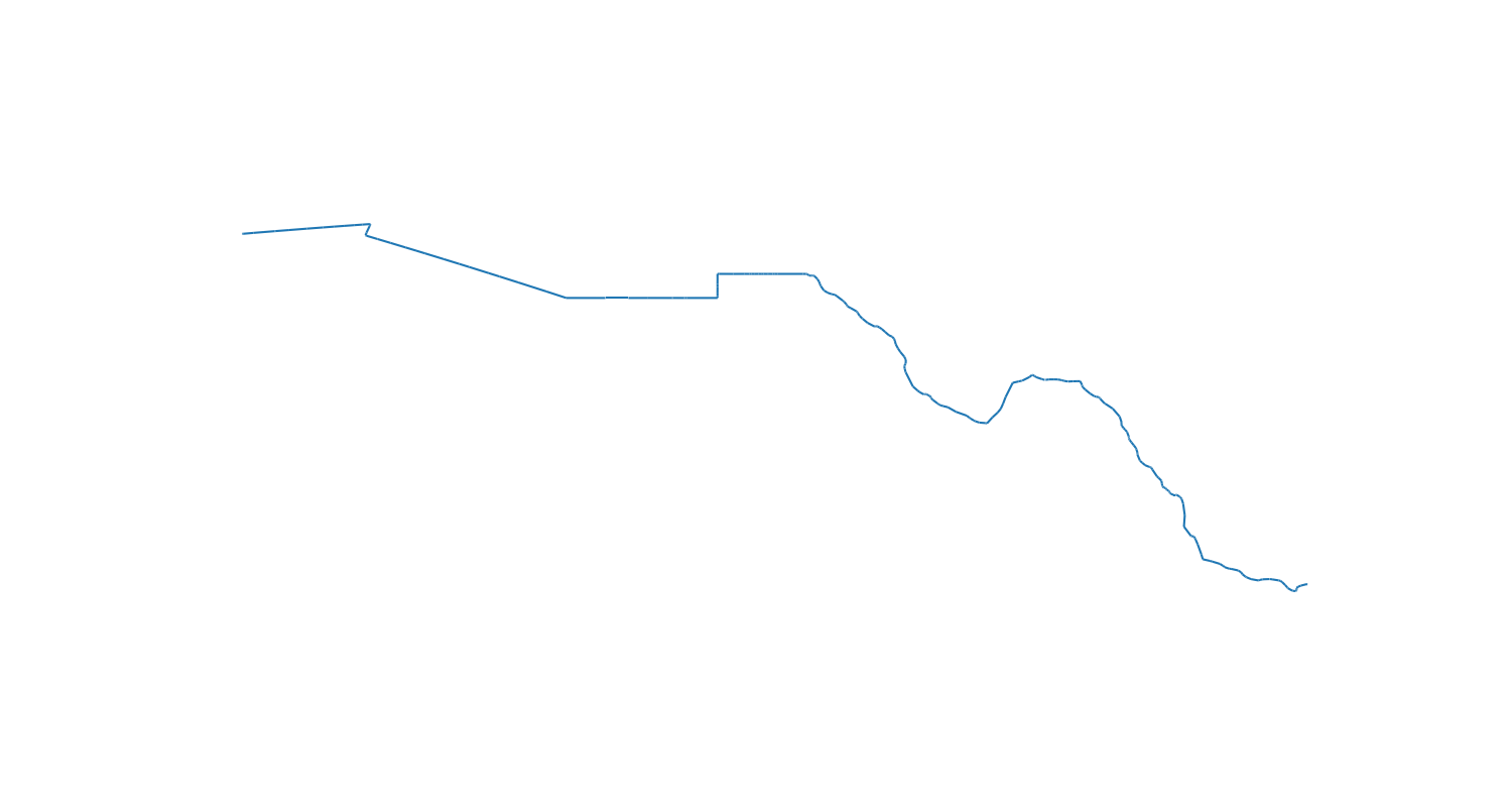
Great! We have ourselves a border!!
Measuring the border
Geodesic Calculations with the Vincenty Equations
As we know from our discussion on the 3(/4) epochs of geodesy, the question of distance along the surface of the earth is not so simple! To illustrate the scale of the problem, measuring this border using a Spherical distance gives us an error of about 1 km (which doesn’t sound too bad, but is a pretty big gap in a wall…), a local projection (Lambert Conic) gives us an error of about 110 km (because the USA is very big) and the global mercator projection puts us out by about 400 km!!!
Clearly, we don’t want any errors like that in our analysis, so we will be using the ellipsoidal distance calculations. These are extremely complex (if you are interested, you can see my version of the code for these calculations (along with the calculation of the above values) here), and involve complex maths that would distract from the purpose of this course. This is, therefore, a good example of a time when it is appropriate for us to use a library: pyproj. As with shapely, pyproj is also built into geopandas, and is also an interface to a C library (simply called Proj), so it will give us a more efficient implementation of these complex mathematical procedures than a pure Python implementation (like mine).
Add the below two snippets to your code in the right place (remember that imports should be collected right at the top!).
from pyproj import Geod
# set which ellipsoid you would like to use
g = Geod(ellps='WGS84')
This function creates a Geod object (short for Geodesy) based on WGS84, which is a very common general model of the shape of the earth (used in the GPS system amongst other things).
This Geod object (which we have stored in the variable g), allows us to make measurements across an ellipsoid, which (as you saw in the lecture) is very important for accurate measurements. Specifically, it gives us access to something called the Vincenty Equations, which are a pair of equations for Geodesic Computations (measuring things on an ellipsoid). If you wish to explore these calculations in more detail, Karney (2013) is a good place to do so, but this is not essential for the practical.
The two equations are known as: forward and inverse. The Forward Vincenty equation (Geod.fwd()) calculates a point on a sphere that is a given distance and direction away from another point (e.g. locate a point 10km due North of my current location). The inverse Vincenty equation (Geod.inv()) calculates the distance and direction between a pair of points (e.g. the distance between your location and my location). As we saw last week, if you move directly from one place to another along a sphere or an ellipsoid, the direction in which you are moving relative to north changes as you move (the blue line in the image below). This is what conformal projections (such as the Mercator - on the right of the image below) seek to correct, by distorting the map to make lines of constant direction (the red line in the image below) appear straight.
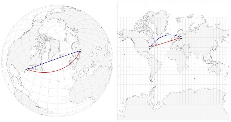
In order to account for this, Geod.inv() returns two directions (which are called azimuths): the forward azimuth, which is the direction in which you would set off from point A to travel directly to point B; and the back azimuth, which is the direction in which you would set off from point B to travel to point A.
The Geod.inv() function therefore works like this:
# calculate the forward and back azimuths and the distance between two point locations
azF, azB, distance = g.inv(start_longitude, start_latitude, end_longitide, end_latitude)
Note that I haven’t asked you to copy and paste this into your code!! If I want you to add a snippet to your code, I will always explicitly say so!
This statement works using variable expansion: the function g.inv() returns a list of three values, which Python expands into three variables for you. If you put only one variable, then it would be populated by a list containing the three values. However, as we are not interested in the forward and back azimuth, however, rather than unnecessarily storing them in variables that we aren’t going to use (azF and azB), we can extract only the distance value by treating it as a list and extracting the value using the index:
# calculate the distance between two point locations
distance = g.inv(start_longitude, start_latitude, end_longitide, end_latitude)[2]
Note that it is the third value in the list that we want, and so we use the corresponding index value of 2 (because list indices start at 0). Also note that all three values are still calculated, we are simply choosing not to store two of them in memory (because we are not using them).
In order to calculate the distance, the function requires four inputs (which are called arguments) - this is simply the two coordinate pairs (remember - longitude is the x coordinate, and latitude is y).
Take a look at the description of
g.inv()in the documentation forpyprojand see if you can understand how it works. It might seem a little unclear at first, but it is really important that you can become familiar with library documentation like this.
Actually measuring the border
Make sure that you understand the use of
g.inv()above, you will need to be able to use it shortly…
Now that we understand how to use g.inv(), we can get on with the tricky business of actually measuring the border… To work out how we might do this, let’s take a look at the coordinates in the border that we calculated earlier:
Run the following snippet after you have calculated the border
print(border)
This should give you something like the below (it will be extremely long!):
MULTILINESTRING ((-97.14073899999994 25.96642900000012, -97.16084299999994 25.96722), (-97.16084299999994 25.96722, -97.265289 25.94110899999998), (-97.265289 25.94110899999998, -97.31529199999994 25.91999800000008), (-97.31529199999994 25.91999800000008, -97.34806799999996 25.89805200000006), (-97.34806799999996 25.89805200000006, -97.34529099999997 25.88805400000007), (-97.34529099999997 25.88805400000007, -97.34278899999998 25.86555499999997), (-97.34278899999998 25.86555499999997, -97.34390299999995 25.858608), (-97.34390299999995 25.858608, -97.34945700000003 25.8488880000001),
What we have there is a MultiLineString, which is made up of a series of segments (each of which is called a LineString) that are defined by a start point and an end point. As you might expect, the end point of one segment will be the same as the start point of then next. You can see this more clearly if we just look at two adjacent segments, one per line:
(-97.14073899999994 25.96642900000012, -97.16084299999994 25.96722)
(-97.16084299999994 25.96722, -97.265289 25.94110899999998)
Can you see how that works? Each is two coordinate pairs, one for the start of the line and one for the end. The end of the first one is the same as the start of the next. If you don’t get it, ask!
To work out the length of the entire border, we simply need to work out the length of each of these segments and add them up, which is where loops come in very handy - all we need to do is loop through each segment, measure the distance between the start point and end point, and add it to a running total (which will be the length of the border after the loop finishes). As luck would have it, we did something very similar in Part 1!
To enable us to loop through the line, we must first convert it to a list of its constituent LineStrings using the .geoms property. We can then access the start and end coordinates of each segment with segment.coords[0] and segment.coords[1] respectively:
Add the below snippet to your code and run it
# loop through each segment in the line and print the coordinates
for segment in border.geoms:
	print(f"from:{segment.coords[0]}\tto:{segment.coords[1]}")
Note: the use of the \t (tab) character to help format the list a little more nicely. This should enable you to see the coordinates for each line segment in the border:
from:(-97.13927161399994, 25.96580638200004)    to:(-97.20494055199987, 25.960638733000067)
from:(-97.20494055199987, 25.960638733000067)   to:(-97.25305130999993, 25.96348093700003)
from:(-97.25305130999993, 25.96348093700003)    to:(-97.26635799199994, 25.960638733000067)
from:(-97.26635799199994, 25.960638733000067)   to:(-97.26920019499994, 25.944360657000047)
from:(-97.26920019499994, 25.944360657000047)   to:(-97.28764868199994, 25.92865102100008)
...
Each coordinate pair here is stored as a tuple (which very similar to a list, except that it is immutable, which means that the elements can’t be edited once they are in there).
To access an individual coordinate from a tuple, you simply use a square bracket to specify the index value, just as you would in a list. However, our segment is represented by a list of tuples, and so we need to use two index references (square brackets, []): one to reference the coordinate pair (start point or end point), and one to reference the coordinate (longitude or latitude). Because the coordinates are stored in the order longitude, latitude, (which isn’t always the case!) the longitude value from the start point (segment.coords[0]) would therefore be segment.coords[0][0], whereas the latitude from the end point (segment.coords[1]) would be segment.coords[1][1], and so on.
Edit your loop (from the above snippet) so that it matches the below. Use the information above to fill in the missing line that will calculate the ellipsoidal distance. To help with this, I have reproduced the earlier example of how to use the
g.inv()function below the snippet - you need to replace each argument with the correct coordinate to get it to work:
# initialise a variable to hold the cumulative length
cumulative_length = 0

# loop through each segment in the line
for segment in border.geoms:

	# THIS LINE NEEDS COMPLETING
	distance =

	# add the distance to our cumulative total
	cumulative_length += distance
Reminder of how g.inv() works:
# how to calculate the distance between two point locations
distance = g.inv(start_longitude, start_latitude, end_longitide, end_latitude)[2]
As you can see, the approach you have taken above is very similar to the one we used to add up the list of numbers in Part 1:
-
Initialise the variable
cumulative_lengthwith the value0 -
Loop through each segment in the border list
-
Measure the length of the segment and add it to
cumulative_lengthwith the increment operator (+=)
At the end of the loop, when each individual segment has been added, the value of cumulative_length will therefore be the length of the border. Simple!
Add a
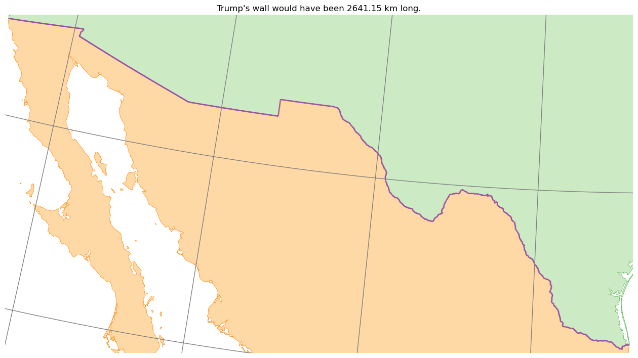
You should have something in the vicinty of 2641152.64 metres (but with more decimal places), if so - well done!
Finishing up
Now we have successfully measured the length of the border, let’s make it into a nice map. To do this, we first need a Projection.
Go to the Map Projection Wizard and select a suitable projection. Given that we are not going to be using this for our calculations (which we did using 3D coordinates), a Conformal projection would be a good option, as this preserves shape (and so will make the countries look as expected).
If all goes to plan, I would expect you to select the Lambert Conformal Conic Projection. Note that we only dealing with data in a small area (North & Central America) this time, so we don’t need to be concerned about the antimeridian wrapping problem!
If you get something different - check with one of the teaching staff
Get the Proj string and store it as a variable called
lambert_conicin your code (remembering that it needs to be surrounded by speech marks ("") to define it as a string.
Now that we have our projection, we can draw our map…
Add the following two snippets to your code at appropriate locations to draw your map. The second snippet should replace the previous code that you used to draw the border.
Also use this opportunity to comment out (
#) or remove any oldprint()statements that you don’t need anymore
# open the graticule dataset
graticule = read_file("../../data/natural-earth/ne_110m_graticules_5.shp")
# create map axis object
my_fig, my_ax = subplots(1, 1, figsize=(16, 10))
# remove axes
my_ax.axis('off')
# set title
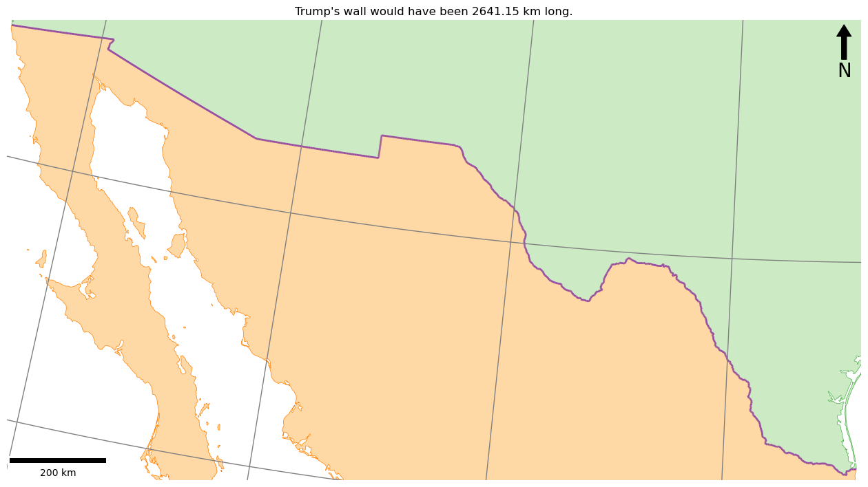
title(f"Trump's wall would have been {cumulative_length / 1000:.2f} km long.")
# project border
border_series = GeoSeries(border, crs=world.crs).to_crs(lambert_conic)
# extract the bounds from the (projected) GeoSeries Object
minx, miny, maxx, maxy = border_series.geometry.iloc[0].bounds
# set bounds (10000m buffer around the border itself, to give us some context)
buffer = 10000
my_ax.set_xlim([minx - buffer, maxx + buffer])
my_ax.set_ylim([miny - buffer, maxy + buffer])
# plot data
usa.to_crs(lambert_conic).plot(
ax = my_ax,
color = '#ccebc5',
edgecolor = '#4daf4a',
linewidth = 0.5,
)
mex.to_crs(lambert_conic).plot(
ax = my_ax,
color = '#fed9a6',
edgecolor = '#ff7f00',
linewidth = 0.5,
)
border_series.plot( # note that this has already been projected above!
ax = my_ax,
color = '#984ea3',
linewidth = 2,
)
graticule.to_crs(lambert_conic).plot(
ax=my_ax,
color='grey',
linewidth = 1,
)
# save the result
savefig('out/2.png', bbox_inches='tight')
print("done!")
Note that now we have had to transform all of our datasets to the Lambert Conformal Conic projection using the .to_crs() function of the GeoDataFrame and GeoSeries objects. Take particular note of how we did this:
border_series = GeoSeries(border, crs=world.crs).to_crs(lambert_conic)
Here we create it as a GeoSeries using the constructor, and set the Coordinate Reference System (CRS) to the same as the one used by the world dataset, before transforming it using .to_crs().
Why did we do this, instead of simply setting the CRS to Lambert Conformal Conic in the first place? Think about it - if the answer isn’t clear to you then be sure to ask, as this is important!
Also take careful note of this snippet from the above:
# extract the bounds from the (projected) GeoSeries Object
minx, miny, maxx, maxy = border_series.geometry.iloc[0].bounds

# set bounds (10000m buffer around the border itself, to give us some context)
buffer = 10000
my_ax.set_xlim([minx - buffer, maxx + buffer])
my_ax.set_ylim([miny - buffer, maxy + buffer])
Here we are setting the bounds of the output map to match the bounds of our border layer, which is necessary otherwise our map would cover the whole world and we wouldn’t be able to see our border at all (comment it out and test it if you don’t believe me!).
In the first line, we are again using variable expansion - .bounds returns a list of four values [minx, miny, maxx, maxy], which Python here is expanding into four variables for us. Alternatively, we could simply store this in a single variable and access each part individually, but this approach is slightly more convenient.
We are then adding a ‘buffer’ of 10km (10,000 m) to each side of the bounds, in order to stop the border touching the edges of the map (which makes it a little more aesthetically pleasing).
Make sure that you understand the above code snippet, and then prove it by tweaking the code to meet your design preferences. Now run the code, you should get an output something like this:
As it is a map, and we’re not animals, we will also add a scalebar and North Arrow.
Add the two snippets below to appropriate locations in script (think about it…) and re-run your code
from matplotlib_scalebar.scalebar import ScaleBar
# add north arrow
x, y, arrow_length = 0.98, 0.99, 0.1
my_ax.annotate('N', xy=(x, y), xytext=(x, y-arrow_length),
	arrowprops=dict(facecolor='black', width=5, headwidth=15),
	ha='center', va='center', fontsize=20, xycoords=my_ax.transAxes)

# add scalebar
my_ax.add_artist(ScaleBar(dx=1, units="m", location="lower left", length_fraction=0.25))
This should have added North arrow and scalebar to your maps as below:
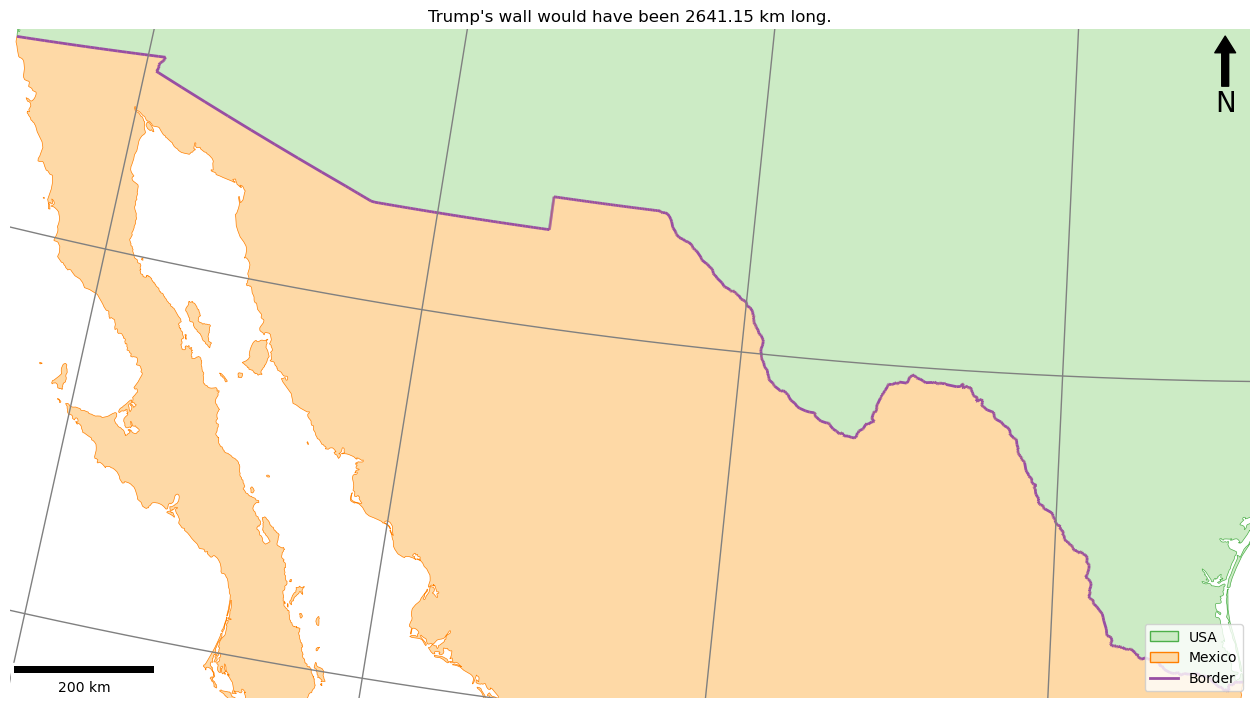
Finally, a map like this would also benefit from a legend, to explain what each symbol refers to. Legends are easy to build, and I am not going to go into detail here as their construction is easily and well explained in the matplotlib legend documentation, guide and this tutorial (amongst others). You should be able to see how it works without too much trouble:
from matplotlib.lines import Line2D
from matplotlib.patches import Patch
# add legend
my_ax.legend(handles=[
        Patch(facecolor='#ccebc5', edgecolor='#4daf4a', label='USA'),
        Patch(facecolor='#fed9a6', edgecolor='#ff7f00', label='Mexico'),
        Line2D([0], [0], color='#984ea3',  lw=0.6, label='Border')
    ],loc='lower right')
Make sure that you understand how the above snippets make the legend in the below map (ask if you aren’t sure!). When you do, add the above snippets to your code at the appropriate locations and run it.
You should now have something that looks like this:
If so, congratulations, you have extracted and measured the ellipsoidal length of an international border! And no distortion error in sight…
Conclusion
We covered a lot this week, but it was worth it - you have learned valuable skills and gained a detailed understanding of two of the fundamental principles of GIS: Topology and Geodesy, as well as implementing them to do a pretty complicated analysis!
See you next week!
A little more…?
Trump never got to the bottom of a design for his wall, and it varies greatly along the sections that are already walled off. Here were some of the designs that were commissioned:
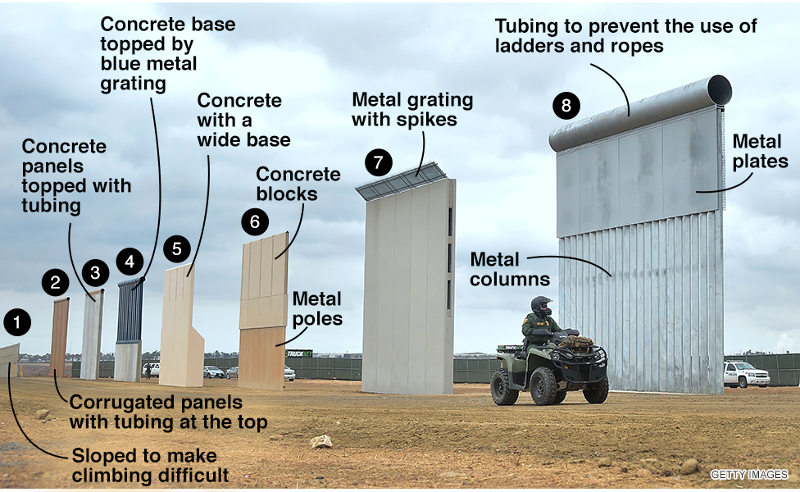
Image Source: BBC News Canada
Let’s say that the wall was to be built with bricks, and would be 10m tall and 2m thick. How many bricks would Trump have needed, and what would be the cost? (you will need to open the link to answer the question…)