"""
Understanding GIS: Practical 2
@author jonnyhuck

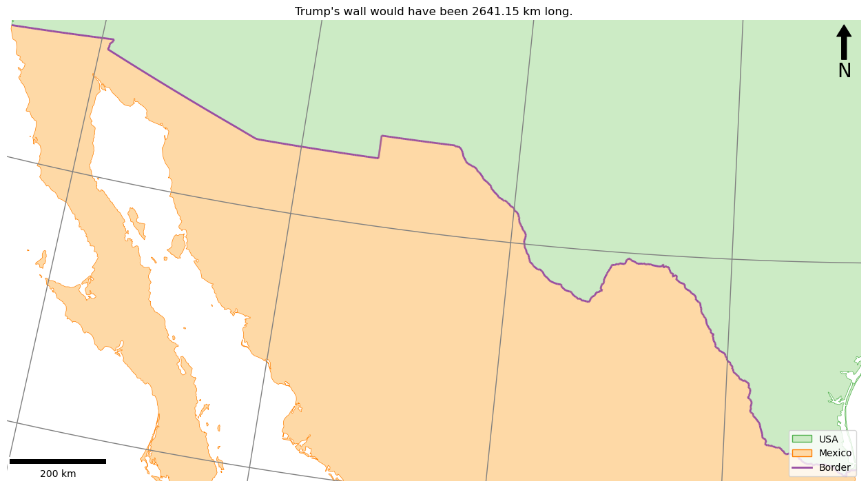
Calculate the length of the border between the USA and Mexico

References:
    http://geopandas.org/reference.html
    https://github.com/ppinard/matplotlib-scalebar
    https://pyproj4.github.io/pyproj/stable/api/geod.html
    https://matplotlib.org/stable/api/_as_gen/matplotlib.pyplot.legend.html
    https://matplotlib.org/stable/tutorials/intermediate/legend_guide.html
    https://matplotlib.org/stable/gallery/text_labels_and_annotations/custom_legends.html

New Topics:
    For Loops
    PyProj
"""

from math import ceil
from pyproj import Geod
from matplotlib.lines import Line2D
from matplotlib.patches import Patch 
from geopandas import read_file, GeoSeries
from matplotlib.pyplot import subplots, savefig
from matplotlib_scalebar.scalebar import ScaleBar

# set which ellipsoid you would like to use
g = Geod(ellps='WGS84')

# load the shapefile of countries
world = read_file("../data/natural-earth/ne_10m_admin_0_countries.shp")
graticule = read_file("../data/natural-earth/ne_110m_graticules_5.shp")
# print(len(world.columns))

# extract the country rows as a GeoDataFrame object with 1 row
usa = world.loc[(world.ISO_A3 == 'USA')]
mex = world.loc[(world.ISO_A3 == 'MEX')]
# print(type(usa))

# extract the geometry columns as a GeoSeries object
usa_col = usa.geometry
mex_col = mex.geometry
# print(type(usa_col))

# extract the geometry objects themselves from the GeoSeries
usa_geom = usa_col.iloc[0]
mex_geom = mex_col.geometry.iloc[0]
# print(type(mex_geom))

# calculate intersection
border = usa_geom.intersection(mex_geom)

# initialise a variable to hold the cumulative length
cumulative_length = 0

# loop through each segment in the line
for segment in border.geoms:

	# calculate the forward azimuth, backward azimuth and direction of the current segment
	distance = g.inv(segment.coords[0][0], segment.coords[0][1],
		segment.coords[1][0], segment.coords[1][1])[2]

	# add the distance to our cumulative total
	cumulative_length += distance

print(cumulative_length)
print(f"Border Length:{cumulative_length:,.2f}m")

''' CALCULATE THE COST '''

# get brick dimensions in metres
brick_length = 215 / 1000
brick_width =  103 / 1000
brick_height = 65  / 1000

# get bricks in each dimension on the wall
n_bricks_long = ceil(cumulative_length / brick_length)
n_bricks_wide = ceil(2 / brick_width)
n_bricks_high = ceil(10 / brick_height)

# get number of bricks in total
n_bricks = n_bricks_long * n_bricks_wide * n_bricks_high
print(f"Number of bricks: {n_bricks:,}")

# get the cost and report
cost = n_bricks * 0.60
print(f"Cost in bricks from B&Q: £{cost:,.2f}")

''' EXPORT THE RESULT TO A MAP '''

# create map axis object
my_fig, my_ax = subplots(1, 1, figsize=(16, 10))

# remove axes
my_ax.axis('off')

# set title
my_ax.set_title(f"Trump's wall would have been {cumulative_length / 1000:.2f} km long.")

# turn border into a GeoSeries and transform to Lambert Conformal Conic projection
lambert_conic = '+proj=lcc +lat_1=20 +lat_2=60 +lat_0=40 +lon_0=-96 +x_0=0 +y_0=0 +datum=NAD83 +units=m +no_defs'
border_series = GeoSeries(border, crs=world.crs).to_crs(lambert_conic)

# extract the bounds from the (projected) GeoSeries Object
minx, miny, maxx, maxy = border_series.geometry.iloc[0].bounds

# set bounds (10000m buffer around the border itself, to give us some context)
buffer = 10000
my_ax.set_xlim([minx - buffer, maxx + buffer])
my_ax.set_ylim([miny - buffer, maxy + buffer])

# plot data
usa.to_crs(lambert_conic).plot(
    ax = my_ax,
    color = '#ccebc5',
    edgecolor = '#4daf4a',
    linewidth = 0.5,
    )
mex.to_crs(lambert_conic).plot(
    ax = my_ax,
    color = '#fed9a6',
    edgecolor = '#ff7f00',
    linewidth = 0.5,
    )
border_series.plot(     # note that this has already been projected above!
    ax = my_ax,
    color = '#984ea3',
    linewidth = 2,
    )
graticule.to_crs(lambert_conic).plot(
    ax=my_ax,
    color='grey',
    linewidth = 1,
    )

# add legend
my_ax.legend(handles=[
        Patch(facecolor='#ccebc5', edgecolor='#4daf4a', label='USA'),
        Patch(facecolor='#fed9a6', edgecolor='#ff7f00', label='Mexico'),
        Line2D([0], [0], color='#984ea3',  lw=2, label='Border')
    ],loc='lower right')

# add north arrow
x, y, arrow_length = 0.98, 0.99, 0.1
my_ax.annotate('N', xy=(x, y), xytext=(x, y-arrow_length),
	arrowprops=dict(facecolor='black', width=5, headwidth=15),
	ha='center', va='center', fontsize=20, xycoords=my_ax.transAxes)

# add scalebar
my_ax.add_artist(ScaleBar(dx=1, units="m", location="lower left", length_fraction=0.25))

# save the result
savefig('out/2.png', bbox_inches='tight')
print("done!")