In which we learn how to use genetic algorithms to solve problems for which we don’t even know the solution! It’s practically magic….

Part 1

Introduction

This week, we are going to take a look at a very different area of computing - one that moves away from our traditional, deterministic “tell the computer to do something and it does it” approach, and towards actually getting the computer to solve problems for us without us needing to explicitly tell it what to do.

This, of course, moves us towards artificial intelligence, which is a huge growth area in the computing industry (and has been for a while) - meaning that it is something that you should be aware of if you want to move into a career in GIS (or indeed, computing more widely).

The problem that we are going to solve this week is one that sounds very simple, but is actually very complicated: we are going to divide a polygon in half. I realise that sounds pretty easy, and it is when you have a simple, regular symmetrical shape like a rectangle, triangle, star or similar. In the real world, however, it is actually quite a major challenge, and the first GIS-based tool for robustly dividing polygons into evenly sized sub-sections was only created for QGIS in 2017 by Jonny Huck!

This solution involves creating a function to assess how good a given solution is (by cutting the polygon in two along a given line and comparing the size of each of the pieces). This function takes one argument, which represents either the x coordinate of a vertical line that is being used to cut the shape (so the argument moves the line side to side), or the y coordinate of a horizontal line (so the argument moves the line up and down). It then uses that function to apply Brent’s Method (Brent, 1973, chapter 4), which locates the root of that function (i.e. the value for the argument that results in the value 0 being returned), as this is the solution! In the QGIS tool, we do this repeatedly to first subdivide the polygon into long strips and then each strip into ‘squareish’ shapes as close as possible to the desired size. You do not need to understand the details of this for this course, but if you are interested, the method is explained in detail in the book and there is even a code implementation in a defunct programming language called ALGOL, which should be quite readable to you as a Python programmer!

Take a quick look at the brent() function in the main Python file in my Polygon Divider plugin.

As you can see, it is quite complex and difficult to understand! This is therefore a situation in which a Genetic Algorithm might well have been a good alternative! Let’s give it a go to solve our problem…

Selecting a Projection

As with all types of analysis, before we start we must first stop to think about the CRS. Because we are dealing with a complex optimisation problem, it will be of great benefit to us to use a projection, as this will simplify the maths and make the algorithm more efficient.

To divide a complex polygon in half, we are obviously dealing with a problem of area (as dividing a polygon “in half” means splitting it into two polygons of equal area). Before we do anything, we will therefore need to select an appropriate equal area projection to use.

Use the Projection Wizard to create an equal area projection suitable for use in Great Britain (you only need to include the mainland!)

Based on the latitude and dimensions of your area of interest, it will likely suggest a Transverse Cylindrical Equal Area map like this (don’t worry if it isn’t exactly the same - it would only be identical to mine if you use an identical bounding box - just be aware that if you use something very different then your coordinates will look different to mine throughout the practical):

+proj=tcea +lon_0=-3 +datum=WGS84 +units=m +no_defs

Create a new file in your week11 directory called week11.py and store your new projection in a variable called uk_ea

Add the below snippet to your code to allow you to import some necessary libraries:

from sys import exit
from geopandas import read_file
from fiona.errors import DriverError

Open the '../data/natural-earth/ne_10m_admin_0_countries.shp' dataset, project it to your new CRS and store it in a variable called world.

A slight diversion: try-except statements

Before we go any further, let’s have a refresh of try-except statements, which we introduced in Week 9. In programming, when something goes wrong, the programming environment (Python in this case) raises an Exception - this is basically a message that something has gone wrong, and it forms the basis of the error messages that you see when you make a mistake in your code.

Normally, exceptions are unexpected, and are resolved by editing your code so that, when the final version is ready, there is no need for your users to ever see them. In some cases, however, exceptions can be triggered in ‘normal’ circumstances, and we (the programmer) need to be able to handle them gracefully in order to make sure that our users do not see a load of messy error messages that make it look like our software is faulty.

Such a situation arises when we open files - a user might give us an incorrect filepath (or move a file to a new location), which would cause an error. In such a case, the code will normally raise an Exception, which will result in an error message appearing. However, if we use a try-except statement, we can catch the Exception and print out a nicer message that won’t scare the user. In other circumstances we might want to run some code if an error happens (for example, when saving a map to a directory, if the directory does not exist then we could create it!).

Let’s have a go,

Replace your read file() statement with the following snippet

# Load the shapefile and project
try:
    world = read_file('../data/natural-earth/ne_10m_admin_0_countries.shp').to_crs(uk_ea)

# if the file does not exist, warn the user  and exit
except DriverError:
    print("Warning, invalid filepath. Exiting.")
    exit()

Can you see how that works? If you put in an incorrect file path, you should now get the message Warning, invalid filepath. Exiting. instead of the whole error message - much nicer!

Test this by making the file path incorrect and running your code.

Finally, extract the feature (row) for the UK (world.ISO_A3 == 'GBR') from the GeoDataFrame and extract the geometry (add a temporary print statement to check that it has worked - you should have a MultiPolygon if all has gone to plan).

Next, we want to get the largest Polygon out of this MultiPolygon, which represents mainland Great Britain. We have done this once before in Practical 4 (Understanding Generalisation), when we approached it like this:

area = 0
for poly in uk.geoms:
    if poly.area > area:
        area = poly.area
        gb = poly

While perfectly valid, I am now going to show you a slightly more elegant and efficient approach to achieving the same thing, using the sorted() function and a lambda function. Here is how they work:

sorted()

sorted() is a function that can sort the items in a list into either smallest-to-largest or largest-to-smallest. For the latter, we simply need to set the reverse argument set to True. Here is an example:

my_list = [9, 4, 6, 3, 2, 7]

# sort the list in reverse order
print(sorted(my_list, reverse=True))

Which would print:

[9, 7, 6, 4, 3, 2]

While this is useful for lists of numbers, if we want to get it to sort something more complicated (e.g. reading the .area property of a geometry object), then we need to give it the capability to access this value. We can do this by passing a function that extracts and returns the .area property of an object, which sorted() will then use in its ranking process. We could just create a function for this and pass it as an argument, like this:

def get_area(poly):
  """
  Extract the area property from the poly object and return it
  """
  return poly.area

# extract the largest polygon (mainland Great Britain)
gb = sorted(uk.geoms, key=get_area, reverse=True)[0]

However, this is an extremely basic operation, which hardly seems to justify building an entire function! Fortunately, Python has a tool up its sleeve for just this situation: the lambda function.

lambda Functions

As an alternative to creating a whole function, we can use a lambda function, which is typically small (normally containing a single expression), anonymous (meaning that we don’t give it a name, so can only use it once) and inline (meaning that we define it in the same line in which we are calling it). They are typically used to perform simple tasks such as this one, without the need to do a full function definition.

A lambda function is written in the form lambda arguments : return statement, here is an example:

# a traditional function to multiply two numbers
def multiply(a, b):
  return a * b

# a lambda function to multiply two numbers
multiply = lambda a, b: a * b

In our case, we want to write a lambda function that will extract the .area property from the polygon geometry and return it. The argument is therefore going to be a geometry object (let’s call it poly) and the return statement is going to be poly.area:

lambda poly: poly.area

Note that in the above snippet poly is simply the variable name and could be switched for any other valid variable name. We have simply used poly because it represents a polygon geometry, and this makes the code more readable.

By using sorted() alongside our lambda function we can therefore sort our polygons in descending order of area, and then take the first one ([0]) from the list to return the largest one (mainland GB)

# extract the largest polygon (mainland Great Britain)
gb = sorted(uk.geoms, key=lambda poly: poly.area, reverse=True)[0]

Implement the above snippet and make a temporary print() statement to test the area - if you got it right then gb should have an area of around 218183218180m².

sorted vs heapq

Last week, we used heapq to optimise sorting a list - whereas this week we are using sorted(). Here is how to decide when to use each of these approaches:

• If it is a single list to which you will repeatedly add and remove elements (like with A*), then heapq is the best choice
• If you are just sorting a list once, then it is as good (and a bit simpler) to use sorted()

In either case, these approaches will be much faster than implementing a sort algorithm yourself (as they are taking advantage of C code, which will run faster than Python).

Now we are ready to get going with our genetic algorithm, but first, back to the lecture…

Part 2

Constructing a genetic algorithm is surprisingly straightforward, and you can control it with a simple list of settings. In your case, they will be as below:

# settings
pop_size                = 50      	# population size
num_parents_mating      = 10      	# mating pool size (how many of the pop get to breed)
threshold               = 0.999   	# the desired precision of the result
mutation_probability    = 0.1     	# probability of a child mutating
max_mutation            = 100000.0 	# 100km max mutation

These settings say that your code will (in order):

• Have a population size of 50 in each generation
• Only the best 10 individuals in each generation get to ‘breed’
• You will keep going until you get to within 0.001% of the perfect result (0.999)
• There is a 10% (0.1) chance that an individual will mutate
• Mutations will move the coordinate by up to 100km (100000m)

Note that there are no ‘correct’ values for these settings. As with most types of artificial intelligence, there is a certain amount of ‘trial and error’ involved with the settings - feel free to play with them and see what happens!

Add the above variables to your code

Creating an initial population

A genetic algorithm is what we might call a stochastic algorithm, because it has random elements in it, meaning that it will not arrive at exactly the same result each time, even if the inputs are identical (as opposed to a deterministic algorithm, where the result is determined by the inputs, and so will always be the same). The weighted redistribution algorithm that you are currently working on for Assessment 2 is another example of a stochastic algorithm, as is the Agent Based Model that we will create next week.

There are several places in a genetic algorithm where we use randomness, the first of which is the initial population, which is created randomly as the first step of the algorithm. As you saw in the lecture, the approach that we are going to take for this problem is to define a random population of cutlines (lines running from East to West, along which we will cut our polygon). The ‘genes’ of each cutline are the binary strings of 0’s and 1’s that define its y coordinate, dictating where between the southern and northern-most extremes of the island they will sit.

Import the following functions from the numpy.random library

from numpy.random import randint, uniform

We are going to represent our random population using a list of objects, meaning that we can set multiple properties for each cutline. We will start by using the uniform function from the numpy.random library - you will remember this from Practical 5: Understanding Distortion.

As you can see in the documentation, the function looks like this:

# calculate a set of sample_number uniformly distributed random numbers between min_value and max_value
random_vals = uniform(low=min_value, high=max_value, size=sample_number)

This produces a numpy array of random numbers using a uniform distribution (meaning that each number is equally as likely to come up) and takes three arguments:

1. low: All values generated will be greater than or equal to low
2. high: All values generated will be less than high
3. size: The number of values that you want to generate

Call uniform, using the pop_size setting (already in your code) and gb.bounds in order to generate a list of the correct number of random numbers that range between the lowest and highest possible y coordinate of your Polygon.

Use a print() statement to test that it has worked.

If it has worked, it should be a list of 50 random numbers (you can check the length using len()) - it will look something like this (remember that this is a stochastic process, so they will not be identical to mine, and they will be different each time you run it):

[6345311.4372485  5781580.97481663 6527419.19447852 6062369.58145342... ]

We will refer to this list of random numbers as our population - it is these values that we are going to ‘breed’ to generate our final result.

We will store our population in a list of dictionaries, which will describe their coordinate value (y) and fitness value (fitness), which will be initialised to None. We could achieve this as below:

# loop through n random numbers
population = []
for y in uniform(low=gb.bounds[1], high=gb.bounds[3], size=pop_size):
  
  # create dictionary and append to the list
  population.append({'y': int(y), 'fitness': None})

However, because this is simply converting one list to another list, we can achieve this much more elegantly using list comprehension.

Convert the above snippet to list comprehension and add to your code, replacing your existing call to uniform (as otherwise you would be doing it twice!).

print() the contents of population to make sure that it has worked

It should look something like this (remember that this is a stochastic process, so they will not be identical):

[{'y': 6431628, 'fitness': None}, {'y': 6408755, 'fitness': None}... ]

Each dictionary object should contain two properties:

• y: the y coordinate for this cutline
• fitness: the score for this individual determined by the fitness function - this is set to None as we haven’t calculated it yet

Creating a Fitness Function

Now we have our population, we must calculate the fitness values of each member in order to determine which are the best individuals, and therefore which get to breed. Our fitness function must take in our population (as a list of objects)

Create a function called get_fitness() that takes in a single argument called population, and add a call to get_fitness() in your main code block that passes in population as the argument and overwrites that same population variable with the result - this should be immediately after you create the population value using list comprehension.

In your get_fitness() function, use a for loop to iterate through each individual in population

Test that it works with a temporary print(individual) statement; remove this statement once that you have verified that it is working

We need to create a measure of fitness for a cutline that is intended to divide a polygon in two. The test should therefore be to divide the polygon along that line and use the ratio of the area of the largest piece to the area of the smallest piece.

Our steps are therefore to:

1. Divide the gb polygon into two smaller polygons using the split function from shapely. We will need to make sure that we don’t end up with more than two polygons by grouping everything above and below the cutline into a MultiPolygon.
2. Work out which ‘half’ is bigger using the argmin function from numpy
3. Divide the area of the larger one by the area of the smaller one - the closer to 1 they are, the better the cutline!

For the first step, we simply need to create a LineString that is a horizontal line running from east to west across the study area at a location dictated by the selected y coordinate. We will achieve this by combining it with the x coordinates from the bounds of gb. We then use that line to split our polygon (using the split() function from shapely), which should produce two or more polygons (depending on the geometry of the polygon that we are dividing). We then pass the result to the group_polygons function, which simply loops through the resulting polygons to check if maximum y value (extracted from the bounding box) is greater than the y value of the cutline. If so, then the polygon is above the cutline, and is added to the top MultiPolygon. If not, then it is below the cutline, and so is added to the bottom MultiPolygon. The two MultiPolygons are then put into a list and returned, meaning that splitting the polygon will always result in no more than two geometries:

from shapely.ops import split
from shapely.geometry import LineString, MultiPolygon

def group_polygons(polys, individual):
    """
    Convert list of polygons into two multipolygons, grouped above and below the cutline.
    """
    # loop through all polygons
    top = []
    bottom = []
    for poly in polys.geoms:

        # if the max y value, it above the cutline, then it is part of the top 'half'
        if poly.bounds[3] > individual['y']:
            top.append(poly)
        
        # otherwise, it is part of the bottom 'half'
        else:
            bottom.append(poly)

    # return list of two multipolygons
    return [MultiPolygon(top), MultiPolygon(bottom)]

# split the polygon into two along the cutline
polys = group_polygons(split(gb, LineString([(gb.bounds[0], individual['y']), (gb.bounds[2], individual['y'])])), individual)

Make sure that you understand how this works and add the above three snippets to your code at the appropriate locations

Secondly, we need to work out which is the larger of the two resulting polygons - fortunately we are now all experts in the use of sorted and lambda functions…

Overwrite the polys variable with a version of itself that is sorted from smallest to largest

Add the below snippet to update the 'fitness' property of the individual dictionary with the ratio between the areas of the smallest and largest polygon:

				# update fitness as ratio of smallest to largest
        individual['fitness'] = polys[0].area / polys[1].area

Finally, return the freshly updated population list (think carefully about the level of indentation that is needed here!)

Test your code using a temporary print() statement for population - if it has worked the fitness values should now be populated in each dictionary in your list

Simulating Evolution

Now we have our population and fitness function, we can start evolving a solution… We will begin by adding a while loop, that will keep going forever until a member of our population gets to within threshold of the target fitness value. We will do this by initialising some variables to keep track of how many generations have gone by (generation), what the fitness score of the current best solution fitness function score is (best_fit), and what the fitness score of the previous best solution was (previous_best_fit)

Add the below snippet to your code:

# initialise loop variables
generation = 0
best_fit = 0
previous_best_fit = None

# loop until we either find a solution within the threshold, or the solutions stop improving
while best_fit < threshold and best_fit != previous_best_fit:

The above snippet will keep looping again and again until one of two things happen:

1. It finds a result within the threshold of the perfect result
2. There is no improvement from one iteration to the next

The first condition is clearly the one that we want, but the second condition is important, as it is possible that we will not be able to reach our threshold, and we will get stuck at a lower value. This means that the loop will also stop if this happens, meaning that we don’t get stuck in an infinite loop!

The first thing that we want to do inside our loop is to extract the parents - these are the individuals that have the highest fitness score

Make a sorted() function to sort population from largest to smallest - you will need a lambda function that returns individual['fitness'] (where individual is the argument). Store the result in a variable called parents.

Add a temporary print statement and exit() to test if this has worked - note that you need the exit() otherwise it will keep running forever!

Once we have sorted our list of objects by fitness value, we will want to extract the top few (a number defined in the num_parents_mating settings variable, 10 at the moment) from our list. The best way to do this is using list slicing, which gives us a way of extracting a set of elements from a list. Here is a reminder of how it works:

# define a list
myList = [1, 2, 3, 4, 5, 6, 7, 8, 9]

# you can extract the start of a list using : and the index of the stopping point
# (from the start to index 5 - the upper limit is tested with < so is not included)
print(myList[:6]) 	# gives 1, 2, 3, 4, 5

# you can extract a set from somewhere in the middle of a list using : and the index of the start and stopping point
# (from index 2 to index 5 - the upper limit is tested with < so is not included)
print(myList[2:6])	# gives 3, 4, 5

# you can extract the end of a list defined using the index of the starting point and :
# (from index 2 to the end)
print(myList[2:]) 	# gives 3, 4, 5, 6, 7, 8, 9 

The combination of the list sort (using sorted() with a lambda function) and list slice give us an efficient approach to extract the required set of parents from our randomly generated population.

Use list slicing to extract the top num_parents_mating (a variable set in your settings variable) from the resulting sorted list - add this to the existing statements so that the result is still stored in the parents variable.

Add a temporary print statement to make sure that you are getting the correct number of individuals back in your list.

If so, you should get a list of 10 objects containing y and fitness properties.

Now we have our parents, we can ‘breed’ them to generate the next generation of our population! We will achieve this using a function called crossover():

Create a function called crossover() with two arguments: parents and offspring_size

To do the crossover, we need to loop through the parents and combine their genes to make a new generation of individuals.

Reminder: Division, modulo and floor division

In the up-coming section, we are going to use two operators that we have not seen since our overview of operators in practical 1: modulo (%) and floor division (//).

The modulo operator (%) does a division but only returns the remainder. For example, 10 % 3 = 1, because three goes into ten three times (3 x 3 = 9), leaving a remainder of 1 (10 - 9 = 1).

Conversely, the floor division operator (//) does a division, but rounds the result down to the nearest whole number (ignoring the remainder). For example, 10 // 3 = 3, because 3 goes into 10 3 times (3 x 3 = 9), leaving a remainder of 1 (10 - 9 = 1) (which is ignored).

We therefore have three variants on division operators in Python - here is a summary of all three:

Right, let’s put these operators to use…

Initialise an empty list called offspring and open a for loop to loop from 0 to offspring_size using range and call the loop variable i.

Inside the loop, we first want to select our parent_1 and parent_2 from the parents pool. To do this, we are going to:

1. Select the parents as the elements from the parents list with indexes equal to i (parent_1) and i+1 (parent_2).
2. Convert the y value from the parent object to a binary string using the bin() function
3. Convert the binary string to a list (so each element is one character, a 0 or 1 in this case)
4. Clip off the first two elements in the list using list slicing (the first two characters are always as 0b and are simply used to signify that it is a binary string - they are not part of the binary string itself)

That sounds like a lot of stuff to do, but it is all achieved in a single line (per parent). Here it is:

# get binary representations of the parents y values
parent_1 = list(bin(parents[i % len(parents)]['y'])[2:])
parent_2 = list(bin(parents[(i+1) % len(parents)]['y'])[2:])

This is necessary as the number of offspring is going to be larger than the number of parents, so we want to be able to keep looping through the parents.

Make sure that you understand what the above snippet does, and then add it to your code.

Once we have the parents, we need to create a new individual by replacing some of the genes from the parent_1 with those from the parent_2 (this would work equally well in the other direction). This is another place where an element of randomness comes into the algorithm, we generate a list of random integers using the randint function from the numpy.random library.

As with uniform, randint has three arguments:

1. low: All values generated will be greater than or equal to low
2. high: All values generated will be less than high
3. size: The number of values that you want

But, for convenience, if we pass only one value and the desired size, then it will default to setting low to 0 and high to the value that you provide.

Add the below snippet to your code to randomly exchange half of the ‘genes’ (bits) between the parents

# swap some random 'genes' (bits) in the binary strings
for r in randint(len(parent_1)-1, size=len(parent_1) // 2):
	parent_1[r] = parent_2[r]

Once the loop is complete, parent_1 contains the genes for the new offspring, which we can convert back from the binary representation to a number with int("".join(parent_1), 2) and then store in a new dictionary and add to our offspring list like this:

# convert back to number and store in a dictionary
offspring.append({'y': int("".join(parent_1), 2), 'fitness': None})

Add the above snippet (after the loop) to add your new ‘child’ to your list of offspring

Now, add a return statement to return offspring, making sure that it is outside both of the for loops!

Back in our main ` while ` loop, we can now call our function in order to generate a new population:

# generate next generation using crossover
population = crossover(parents, pop_size)

Add the above snippet to your code (in the main loop, after the line where you create the parents) in order to call your crossover() function. Use a print statement to check that it has worked

This should, give you a new list containing a population of 50 individuals (the next generation), all with fitness set back to None:

[{'y': 5919825, 'fitness': None}, {'y': 5928648, 'fitness': None}, ...]

Mutation

In any healthy population, there must be mutations (this is where the individual features of a species come from!). In the case of a genetic algorithm, mutations are very important because (as I described in the lecture) they avoid the algorithm getting stuck in local minima (where it thinks it is heading toward the result, but in reality it isn’t).

Once again, we will make a function to handle our mutation, which we will call, er, mutation()…

Create a function called mutation() that takes in three arguments: population, mutation_probability and max_mutation.

In this function, we want to loop along a list of numbers representing the index of the elements in population. We can achieve this in the usual way using range() and len().

Add the loop described above, calling the loop variable i.

Once again, we are adding some randomness to our algorithm here, using uniform to decide whether or not we want to mutate each individual. We have already set the probability that a given individual will mutate with mutation_probability (0.1), so we simply want to get a single random number between 0 and 1 and see if is smaller than the specified probability - if it is, then we mutate; if not, then we don’t!

If we do want to mutate, then we use uniform to add a random offset (between -max_mutation and max_mutation) to the y property of the current object.

Read the below snippet and make sure that you understand it, then add it to your code to complete the above steps.

# does this child want to mutate?
if (uniform() < mutation_probability):

  # apply the random value as a mutation to the child
	population[i]['y'] += int(uniform(-max_mutation, max_mutation))

Add a return statement (at the appropriate indentation level) to return the modified (mutated) population list.

Back in your main code block, add a function call to mutation that passes population, mutation_probability and max_mutation as arguments. Overwrite the population variable with the result.

Once again, test the output using a temporary print() statement

The result should be a very similar list to the one in offspring_crossover (except approximately 10% of them will have changed!).

Assessing your New Population

Now that we have our new population, it’s time to see how good they are…

Calculate the fitness of your new population. Overwrite the population variable with the result.

Now we have three lines, all of which overwrite the same variable (population).

Replace those three lines (all of the lines inside the loop) with one single statement as per the below snippet:

# get the next generation, mutate and update fitness values
population = get_fitness(mutation(crossover(parents, pop_size), mutation_probability, max_mutation))

WARNING: make sure that you replace the other lines with the above, and don’t add it as well - otherwise this will duplicate the work and slow down your code!

Now we can use the same trick as before to sort our population by fitness and clip off the best one using list slicing. We can also increment our generation counter and report how many generations there have been and the current best fitness value.

# get the current best individual
best_match = sorted(population, key=lambda individual: individual['fitness'], reverse=True)[0]
previous_best_fit = best_fit
best_fit = best_match['fitness']

# increment generation counter and report current fitness (1 = perfect)
generation += 1
print(f"\tgeneration {generation}: {best_fit}")

Add the above snippet to your code

And with that, we have completed our loop! It will run until the result reaches the required threshold (0.999, or within 0.1% of perfect), at which point, we have our result stored in best_match!

After the loop has completed, report your result with the below snippet:

# report the best match and output
print(f"Best solution : {best_match['y']} (fitness: {best_match['fitness']} generations: {generation})")

Creating an Output

Now we have our result, all that remains is to map it!

Create a LineString object to represent your cutline (if you get stuck, take a look at the get_fitness function…), store the result in a variable called cutline

Use cutline to divide gb into two polygons (remember to group_polygons()!) and store the result in a variable called polys

Add the below snippets to draw your results to a map:

from geopandas import GeoSeries
from matplotlib.patches import Patch
from matplotlib_scalebar.scalebar import ScaleBar
from shapely.geometry import LineString, MultiPolygon
from matplotlib.pyplot import subplots, savefig, Line2D

# setup figure for output
fig, my_ax = subplots(1, 1, figsize=(16, 10))
my_ax.axis('off')
my_ax.set_title("The North-South Divide")

# add layers
GeoSeries(polys[0], crs=uk_ea).plot(
    ax = my_ax,
    color = '#ccebc5',
    edgecolor = '#4daf4a',
    linewidth = 0.3
    )
GeoSeries(polys[1], crs=uk_ea).plot(
    ax = my_ax,
    color = '#b3cde3',
    edgecolor = '#377eb8',
    linewidth = 0.3
    )
GeoSeries(cutline, crs=uk_ea).plot(
    ax = my_ax,
    color = '#e41a1c',
    linewidth = 1
    )

# manually draw a legend
my_ax.legend([
    Patch(facecolor='#ccebc5', edgecolor='#4daf4a', label='The North'),
    Patch(facecolor='#b3cde3', edgecolor='#377eb8', label='The South'),
	Line2D([0], [0], color='#e41a1c', lw=1)],
	['The North', 'The South', 'Cutline'], loc='lower right')

# add north arrow
x, y, arrow_length = 0.98, 0.99, 0.1
my_ax.annotate('N', xy=(x, y), xytext=(x, y-arrow_length),
	arrowprops=dict(facecolor='black', width=5, headwidth=15),
	ha='center', va='center', fontsize=20, xycoords=my_ax.transAxes)

# add scalebar
my_ax.add_artist(ScaleBar(dx=1, units="m", location="lower left"))

# store image
savefig("./out/9.png", bbox_inches='tight')
print("done!")

If all has gone to plan, you should have something like this:

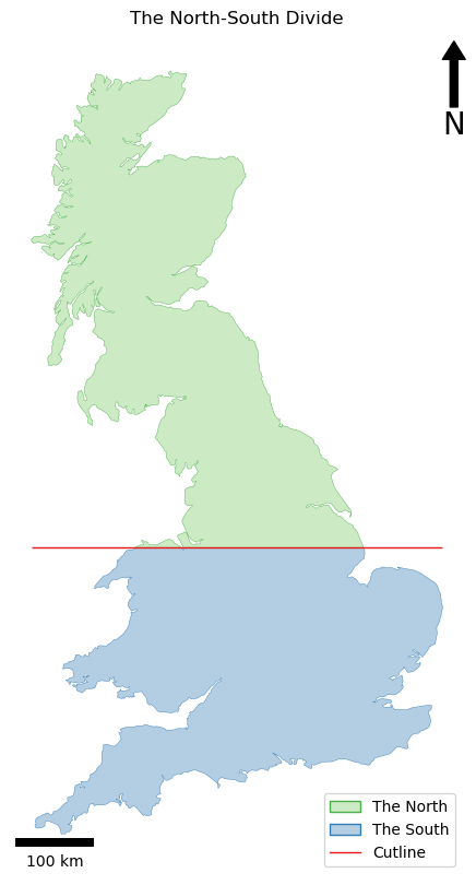
…and your output should be something like this:

        generation 1: 0.9265359555389336
        generation 2: 0.9370288363218718
        generation 3: 0.9991685144734718
Best solution : 5928743 (fitness: 0.9991685144734718 generations: 3)
done!

Remember that your result will not be exactly the same as mine, or between individual runs of your own code - this is perfectly normal and acceptable for a stochastic algorithm! Your code could take any number of attempts to find the answer!

As you can see, it got to within 0.1% (0.001) of the perfect result in only three generations - not bad!!

A little more…?

If you want to keep going, try and make a version that separates east and West, rather than North and South, or if you are feeling really adventurous, try and split the island into thirds!