In which we learn about Graph Theory, examine the Seven Bridges of Königsberg, and implement your own routing algorithm

Part 1

The Seven Bridges of Königsberg

As you have seen in the lecture, graph theory is important to several areas of GIS, and so is important for you to understand as well. To get used to graph theory, we are going to start with a short exercise that tests Leonhard Euler’s assertion that it is impossible to tour the city of Königsberg, crossing each bridge exactly once, and returning to the same point. Let’s remind ourselves of the story…:

(comic by Matteo Farinella)

Can we prove this using Python? Let’s find out…

We are going to use a Python library called networkx, which is specifically designed to help with graph or network-based analyses. What we are going to do is simply:

1. Create a graph in Python that represents Königsberg in 1736.
2. Test to see whether or not it is Eulerian (that is, whether or not it can be completely traversed by visiting each edge only once).

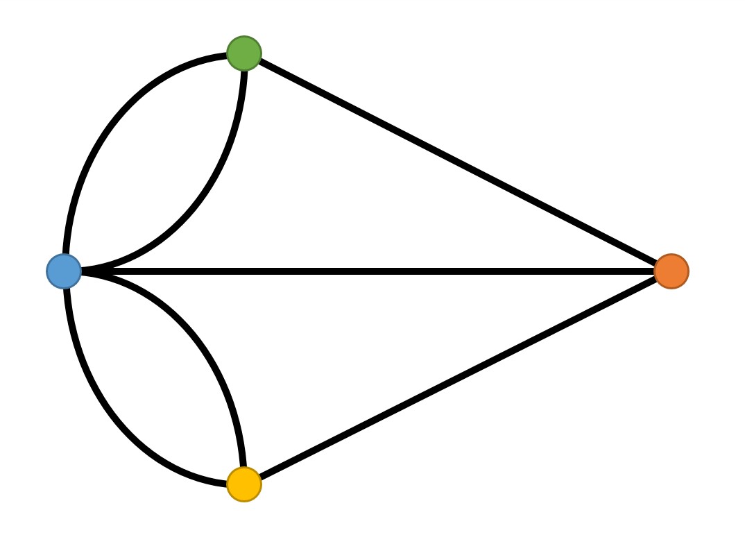
Like Euler, we are going to take the above map of Königsberg and convert it to a topological representation, like this:

Making a Graph in Python

Let’s get to it then. All we need is to import the Graph class from networkx into our code, and then use some simple functions that networkx provide for us to easily make a graph.

# Import the library
from networkx import Graph

# Create a graph object
graph = Graph()

# Add a node to the graph
graph.add_node(id)

# Add an edge to the graph
graph.add_edge(node_id1, node_id2)

In the case of our seven bridges example, therefore, we need to do something like this:

from networkx import Graph

# Create a graph object
graph = Graph()

# Add the 4 islands (nodes), colours as per the above diagram
graph.add_node('Blue')
graph.add_node('Green')

# Add the 7 bridges (edges), colours as per the above diagram
graph.add_edge('Blue','Green')	# e.g. this is a bridge from the Blue to Green island
graph.add_edge('Green','Blue')

# Print a report about the graph that you have just made
print(f"We have {len(list(graph.edges()))} bridges between {len(list(graph.nodes()))} islands.")

Simple! Right?

Paste the above snippet into a new file in your week10 directory called sevenbridges.py.

Add the 2 missing graph.add_node() and 5 missing graph.add_edge() statements to match the above diagram.

Run the file.

If all has gone to plan, you should get something like this:

"We have 5 bridges between 4 islands."

Eh?

How have we got 5 bridges when we have clearly set 7 in the code above? Well, it’s actually quite simple, networkx is trying to be helpful, and remove any duplicate edges that we may have added by mistake. Ordinarily this could be quite a useful feature, but not in this case, so we need to do something about it.

Fortunately, this is quite easy, all we need to do is change the type of graph to one that allows this (a MultiGraph), and then add something in there to differentiate the bridges (edges) from each other. We can do this with an attribute, which could be used to store details about an edge (or node, if you wish) such as its length, speed limit, name etc. In this case, we do not need the attribute to refer to anything in particular, so we can simply number the bridges. Here’s how:

Update graph so that it is a MultiGraph (remember the import statement) - this is a type of graph that can handle the difference.

Then, add an unique 'id' attribute to each edge as per the below example:

graph.add_edge('Blue','Green', id=1)

Which gives:

"We have 7 bridges between 4 islands."

Much more like it!

Now we have our graph, it’s time to test whether it is Eulerian or not. If we wanted to do a brute force approach to this, it would take a very long time:

gif by brilliant.org

However, thanks to Euler, we can use a much neater rule to test for this:

• For a graph to be Eulerian (i.e. you can traverse every edge exactly once and end up back at the starting node), every node must have an even degree (i.e. each node must be connected and have an even number of edges connected to it). The route taken would be referred to as a Eulerian Circuit.
• For a graph to be semi-Eulerian (i.e. you can traverse every edge exactly once, but end up at a different node), there must be exactly two nodes of odd degree (that is, each node must be connected and two of them can have an odd number of edges attached to them - these will be the start and end of the route). The route taken would be referred to as a Eulerian Path.

As you can imagine this is much easier to test! It would be trivial to do this ourselves, but networkx already has a simple function built in for this (and pretty much any other network analysis algorithm that you can think of):

from networkx import is_eulerian

# Returns True or False to describe whether or not the graph is Eulerian
is_eulerian(graph)

Add the above snippet as the conditional test in an if-else statement to your code in order to report whether or not the graph is Eulerian. If it goes well, you should end up with something like this:

"We have 7 bridges between 4 islands."
"The graph IS NOT Eulerian."

We have programmatically confirmed that Euler was correct, and learned to make a graph at the same time!

Have a play with your graph and see if you can re-design Königsberg so that it does form a Eulerian circuit.

If you manage it, you can get networkx to calculate the route for you:

from networkx import eulerian_circuit

# Return the Eulerian route around Kaliningrad
print(list(eulerian_circuit(graph)))

Add the above snippet to print the route of the Eulerian Circuit around the graph.

Nice work! Now back to the lecture…

Part 2

The A* Shortest Path Algorithm

Things have, changed somewhat since 1735, and one of the big changes is that Königsberg is now called Kaliningrad, located in an enclave between Poland and Lithuania. Now we are able to use graph theory to analyse a network, we are finally able to do what all of our non-GIS friends* think we do all the time anyway: build a ‘SatNav’!

*(that is, if anyone has non-GIS friends - of course, I wouldn’t advise it…)

Specifically, we will be implementing the A* shortest path algorithm - which is a relatively simple but highly efficient routing algorithm by Hart et al (1968). As we saw in the lecture, this algorithm was not created for the field of GIS, but rather for robotics, as a way of guiding Shakey the Robot - this is considered to be one of the first applications of Artificial Intelligence.

Pseudocode

This algorithm is quite complicated, so to avoid confusion, I am going to provide a pseudocode overview for you before we get stuck in:

initialise a dictionary of parents for each node, where a node's parent is the one before it in the shortest path so far (parents)

initialise a heap queue and load the start node into it (queue)

while there are still nodes in queue:
	
	get the current node (node)
	
	if node is the end of the path: 
		return the path

	if we have assessed node before:
		if it is the start node or one to which we have already found a shorter route:
			skip to next node in the queue
	
	store the parent of node into parents
	
	for each neighbour of the current node (neighbour):
	
		get the network distance from the start of the path to neighbour using the heuristic function (d1)
		
		if we have assessed neighbour before and have already found a shorter route to neighbour:
			skip to next node in the queue
		
		get the straight line distance distance from this neighbour to the end using the heuristic function (d2)
		
		calculate the estimated distance for a route through neighbour (d3)
		
		load neighbour into the queue, with d3 as the priority

This loop will continue until it either finds the route, or runs out of nodes in the queue (meaning that no route is possible).

Got it? Right, let’s get to it…

Create a new Python file called week10.py

We are going to use a graph constructed from the freely available data at OpenStreetMap. To save us some time, I have downloaded this for you, and you can access it (along with some background data for drawing a map later) in your ../data/kaliningrad/ directory.

Manually making a graph out of GIS data can be a rather dull and long-winded process, and is not one that I think there is a great deal of value in us doing (you already know how to make a graph from Part 1, and parsing OSM data is not a very exciting way to spend a Tuesday morning…). Fortunately, there is a library that can handle this for us called osmnx - basically, it simply loads each section of road as an edge, with a node at each junction - simple!

Import the graph_from_xml() function from osmnx as per the below:

from osmnx import graph_from_xml

We can now load our data (currently in OpenStreetMap XML format) into a MultiDiGraph (like a MultiGraph, but allows one way streets) using the convenient functionality of osmnx:

# create a MultiDiGraph from an XML dataset from OpenStreetMap
graph = graph_from_xml('../data/kaliningrad/kaliningrad.xml')

Add the above snippet to your code and run it to make sure that you don’t have any errors - remember, you have not asked it to output anything, so we are expecting no output unless something has gone wrong!

Oh no! Something has gone wrong. If you’re working on Windows, it is highly likely that you have encountered an error when trying to run the above code snippet (UnicodeDecodeError: 'charmap' codec can't decode byte 0x81 in position 5500: character maps to <undefined>). The problem here occurs because of a mismatch between the encoding system of the file, which uses utf-8, and the encoding system that graph_from_xml is trying to use, which is called cp1252. Because computers can only think in terms of numbers, when working with strings, they need to use an encoding system to define which character (i.e., letters, numbers, symbols etc.) should be represented by each number. This is called a character map (‘charmap’ in the above error message) and is simply a list of numbers and their corresponding characters, like this one. Rather than just working with just one, Operating Systems will include many different character encoding systems, which is good because it means that the same Operating System can be used in many different languages without needing adjustments to the underlying code. However, this also means that your software needs to know which character map to use when reading a text file, otherwise it will either return nonsense or (as in this case) cause an error (think of it as like trying to read Braille using the rules for Morse code.).

Unfortunately, there is currently a bug in the latest versions of osmnx that is causing Windows machines to try to interpret our xml file using the wrong character map (cp1252 rather than utf-8), even though the XML file contains a line specifying that it is encoded in UTF-8. Even worse, because the graph_from_xml() function in the osmnx library has no option for the user to specify the encoding system that we want to use, there is nothing much that we can do about it! In fact, that’s not strictly true, because osmnx is open-source which means we can easily inspect the underlying code, in this case on Github. This allows us to critically assess the underlying algorithms and their implementation, as we are encouraging you to do throughout the course, as well as modify the code and suggest improvements by opening issues, which is what we’ve done when encountering this error - see here!

For now, this is an issue we just need to work around. For Windows users, please download (and unzip) a new version of kaliningrid.xml here, which is stored with cp1252 encoding, making sure to use this file for the remainder of the practical.

Building a Spatial Index for your MultiDiGraph

Now we have a MultiDiGraph, we just need to do one more step of data processing before we can start our analysis - we need to build a Spatial Index. In practical 3, we learned to make spatial indexes manually, even though geopandas can do it for us. For example, we did this for a “extract all of the points within a polygon” operation:

# construct a spatial index
idx = Index()
for id, point in points.iterrows():
	idx.insert(id, point.geometry.bounds)
  
# filter the dataset using the spatial index
possible_matches = points.iloc[list(idx.intersection(polygon.bounds))]

# get the points within the polygon using a topological test
precise_matches = possible_matches.loc[possible_matches.within(polygon)]

However, (and as I briefly explained here) this instance, geopandas would actually have used a spatial index for us (using the one in the .shx file), so we could have just done this, which takes roughly the same amount of time to run:

precise_matches = points.loc[points.within(polygon)]

However, doing this would have two problems:

1. We would not understand how spatial indexes work in the same level of detail (which is the point of the course…)
2. We would only be able to use spatial indexes when dealing with a GeoDataFrame (as opposed to when working with raw geometries, data in other formats, or graphs…)

Problem 2 is particularly pertinent here, as we are now in a situation where we desperately need a spatial index to enable us to efficiently work out the nearest node in the graph to our specified start and end points - these will be the actual start and end points for our route. Fortunately - because we know how to use rtree, this is no problem for us:

from rtree.index import Index

# create spatial index from graph
idx = Index()
for id, data in list(graph.nodes(data=True)):
  idx.insert(	# MISSING LINE

Copy, paste and complete the above snippets to initialise a spatial index loop through the nodes in your graph object. Complete the missing line to build your spatial index. You can use the below hints to help you:

• Remember that the Index() constructor takes two arguments, an id and the bounding box:
  • You will need to convert id to a number using int(id) to be able to use it as the label in the spatial index.
  • Remember that the coordinates for the bounding box are passed as a tuple in the form (x, y, x, y)
• If you print() the data variable, you will see that it is a dictionary (key:value pairs listed within curly braces { }), and you should be able to see how to extract the x and y coordinates from the dictionary to make your bounding boxes. Remember, a dictionary is a collection of key:value pairs. For example:

my_dictionary = {'an_item': 1, 'another_item': 'a value'}
print(my_dictionary['another_item'])

a value

• You can always check out the rtree documentation for more assistance.

Note how you have to pass the named argument data=True to the graph.nodes() function - if you don’t do this then it will not include the coordinates! Note that we have used the id from the graph as the id in the spatial index - this enables us to be able to tell which entry in the spatial index refers to which node in the graph (as they both have the same id)!

To make sure that this has worked, we can do a simple test:

Use the below snippet to test the number of entries in your Index against the number of nodes in your Graph:

print(idx.count(idx.bounds), len(graph.nodes))

If it has worked, the numbers should be the same!

Now we have our graph (graph) and spatial index (idx), we can use the spatial index to efficiently locate the nearest node in the graph to the start and end point of our route using the .nearest() function just as we did in practical 3:

# specify the start and end point of your route
from_point = (20.483322,54.692934)
to_point = (20.544863,54.723827)

# calculate the 'from' and 'to' node as the nearest to the specified coordinates
from_node = list(idx.nearest(from_point, 1))[0]
to_node = list(idx.nearest(to_point, 1))[0]

# print the 'from' and 'to' nodes to the console
print(graph.nodes()[from_node], graph.nodes()[to_node])

Add the above snippet to your code and run it

If all has gone to plan, you should have the following nodes as the start and end points of your route:

{'y': 54.6950447, 'x': 20.4841665} {'y': 54.7242909, 'x': 20.5442207}

Defining your heuristic

Now we have two nodes in the graph, all we need to do is find the shortest path between them. Of course, networkx has all of the major routing algorithms built right into it , but simply using them will not really help us to understand how they work - so we will create our own!

As you will remember from the lecture, we will be using the A* routing algorithm (Hart et al. 1968), which is an example of an heuristic routing algorithm. Heuristic is a word that comes up quite a lot in computing, especially in optimisation algorithms (like finding the shortest path). Simply, an heuristic function is one that ranks alternative approaches according to some sort of measure (distance in our case, as we are looking for the shortest path).

To be able to use distance in this way, we will need a function that is capable of:

1. taking in two nodes and extracting their geographical coordinates
2. calculating the distance between them.

As our dataset is in wgs84 (geographical) coordinates, we will use pyproj.Geod.inv() for our distance measurement, just like in Practical 2 and Assessment 1.

Add the below snippets at the appropriate locations in your code, and complete them to permit the measurement of a distance between two nodes in the graph (remember that you know how to extract coordinates from a node from the above section)

from pyproj import Geod

def ellipsoidal_distance(node_a, node_b):
	"""
	Calculate the 'as the crow flies' distance between two nodes in a graph using
	 the Inverse Vincenty method, via the PyProj library.
	"""
	# extract the data (the coordinates) from node_a and node_b
	point_a = graph.nodes(data=True)[node_a]
	point_b = # MISSING LINE

	# compute the distance across the WGS84 ellipsoid (the one used by the dataset)
	return Geod(ellps='WGS84').inv(point_a['x'], point_a['y'], point_b['x'], point_b['y'])[2]

Test the above function by adding a temporary print statement that makes a call to ellipsoidal_distance() between from_node and to_node

If it went well, you should have something like:

5057.9m

Remember to remove this print statement once you are satisfied that it works

Route Reconstruction

As you saw in the lecture, the A* algorithm uses the heuristic function to searches through a graph until it reaches the desired target node (i.e. the end of the route) - as it goes, it effectively keeps ‘notes’ of which nodes it has visited, and which came before them. Once it finds the end point, it then uses those ‘notes’ to reconstruct the shortest path that it found; which it achieves by looping backwards through the notes that it has made until it finds its way back to the start.

We will use a simple function to achieve this:

def reconstruct_path(end_node, parent_node, parents):
	"""
	Once we have found the end node of our route, reconstruct the shortest path 
	 to it using the parents list
	"""
	# initialise a list that will contain the path, beginning with the current node (the end of the route)
	path = [end_node]
	
	# then get the parent (the node from which we arrived at the end of the route)
	node = parent_node

	# loop back through the list of explored nodes until we reach the start node (the one where parent == None)
	while node is not None:

		# for each node in the path, add it to the path...
		path.append(node)

		# ...and move on to its parent (the one before it in the path)
		node = parents[node]
	
	# finally, reverse the path (so it goes start -> end) and return it
	path.reverse()	# note that this is an 'in place' function that edits the list itself, it does not return anything!
	return path

In this function we have three arguments:

• end_node: the end node in the path
• parent_node: the node from which we arrived at the end node
• parents: a dictionary that contains the parent node of each node that we searched

We then loop back through our route, getting the parent of each node that we reach dictionary - starting with the end node, we:

1. add it to a list that will describe our path (path.append(node))
2. move to the parent node that we stored for it (node = parents[node])
3. repeat until we get to a node with no parent (which is the start node!)

Then we simply reverse the order of the list (as it currently goes end → start) with path.reverse()and return it - simple! Note, however that path.reverse() is a rather unusual function in that it is an in place function, meaning that it edits the object itself, rather than returning anything. if you tried to do path = path.reverse() or return path.reverse() then you would simply get None, as the function does not return anything!

Make sure that you understand this and then add the above function to your code at an appropriate location

The A* Algorithm

Now that we have our heuristic function in place, we can start making our routing algorithm:

# calculate the shortest path across the network
shortest_path = astar_path(graph, from_node, to_node, ellipsoidal_distance)

Add the above snippet to your code (think about where it should go…)

Make the definition statement for the astar_path() function, name the four arguments G, source, target and heuristic

Note that here we are passing a function as the fourth argument! This is a little unusual in traditional object oriented programming, but perfectly acceptable in Python (a feature borrowed from functional programming approaches)!

A slight diversion: try-except statements

Before we go any further, there is something that we need to consider. In programming, when something goes wrong, the programming environment (Python in this case) raises an Exception - this is basically a message that something has gone wrong, and it forms the basis of the error messages that you see when you make a mistake in your code.

Normally, exceptions are unexpected, and are resolved by editing your code so that, when the final version is ready, there is no need for your users to ever see them. In some cases, however, exceptions can be triggered in ‘normal’ circumstances, and we (the programmer) need to be able to handle them gracefully in order to make sure that our users do not see a load of messy error messages that make it look like our software is faulty.

Such a situation arises when calculating routes: If we are not able to calculate a route (normally because it is not possible, such as if you wanted to go from one side of a river to another but there was no bridge), then we should raise an Exception describing the problem. You will have seen many such exceptions in error messages during the course so far, such as:

• NameError: when you refer to a variable that does not exist
• IndexError: when you try to read a value from a collection that does not exist
• IndentationError: when you have mixed up tabs and spaces in your indentation

Conveniently, networkx contains exceptions that we can use: NetworkXNoPath, indicating that no path can be found; and NodeNotFound, indicating that one of the nodes specified in the function (from_node or to_node does not exist in the graph). We will use conditional statements to seek out these situations in our function and raise these exceptions if they occur. We can then catch these exceptions, and provide a nice message to our user explaining the issue (rather than revealing a terrifying Python error message). This is achieved using a try-except statement, in which we ask Python to try a block of code, and in the event that an Exception is raised from it, it will stop what it is doing and run a different block of code that is identified by the keyword except.

This sounds complex but is actually very simple, here is how we would apply it to our route calculation:

from sys import exit
from networkx import NodeNotFound, NetworkXNoPath

# use try statement to catch exceptions
try:
	# calculate the shortest path across the network
	shortest_path = astar_path(graph, from_node, to_node, ellipsoidal_distance)

# catch exception for no path available
except NodeNotFound:
	print("Sorry, there is no path between those locations in the provided network")
	exit()

# catch exception for no path available
except NetworkXNoPath:
	print("Sorry, there is no path between those locations in the provided network")
	exit()

Can you see how that works? We have moved our astar_path function into the try block (as this has the potential to raise a NetworkXNoPath or a NodeNotFound Exception), and then if this Exception does happen, we deal with it by printing a message for the user and then exiting the program gracefully. Note how you can have multiple except statements to deal with different types of errors.

Update your call to astar_path() so that it incorporates the above try-except statement

Now that we are ready to catch some exceptions, we can start raising them:

Add the below snippet to your astar_path() function:

	# first, make sure that both the `source` and `target` nodes actually exist...
	if source not in G or target not in G:
		raise NodeNotFound(f"Either source ({source}) or target ({target}) is not in the graph")

As you can see, this checks that both of your nodes (source and target) are in the graph (G) - if not, then we will raise an exception, which will exit the function and trigger the contents of the relevant except block that you created above. If we had not created an except block, then it would simply exit the code and print an error message the console like it does with other types of error.

Let’s test this:

Change your call to astar_path() to the below - this asks for a route between two nodes that do not exist - then run your code

shortest_path = astar_path(graph, 1, 2, ellipsoidal_distance)

If all goes to plan, you should get a nice user-friendly message, rather than a Python error message:

Sorry, there is no path between those locations in the provided network

Lovely!

Restore your call to astar_path() back to how it should be:

astar_path(graph, from_node, to_node, ellipsoidal_distance)

Implementing a Heap Queue with heapq

As you saw in the lecture, the performance of the A* algorithm is based upon on its ability to rapidly sort a list of previously assessed nodes. In order to do this, we will use the heapq library, which is built in to Python, and provides an implementation of the heap queue algorithm. This allow us to store data in a binary tree (similar to an RTree), in which each parent node has a value smaller than its child node (whereas in an RTree, each parent node’s bounding box contains the bounding box of the child node).

Whereas in a list, the .pop() function would simply remove the first element in the list and retuern it to you; the heappop() function of a heapq will return the feature with the smallest value (as elements in a heapq are stored in size order). This is therefore an extremely efficient data structure in situations where you require data to be stored in size order - far better than using a standard Python Collection and repeatedly sorting it (which is quite a computationally intensive task)!

To illustrate, here is an example of some simple numeric values in a heapq (think of it as a tree structure - where each number is the child of a smaller number):

                               0

              1                                 2

      3               4                5               6

  7       8       9       10      11      12      13      14

15 16   17 18   19 20   21 22   23 24   25 26   27 28   29 30

Can you see how that works? As you add new objects to it using heappush() (the equivalent of .append() for a list), they will be stored in a way that maintains the size ordering, meaning that you never have to sort your data! These structures are widely used for a wide variety of applications including task scheduling, simulation and (of course) route optimisation!

When we have tree structures like this, we normally refer to higher elements in the structure as being the parent of lower elements (the child). For example, 0 is the parent of 1, whereas 1 is the parent of 4 etc…

Add the following statements to import the necessary functions from the heapq library

from heapq import heappush, heappop

Now add the below snippet to your astar_path() function:

	# create a counter to prevent to ensure that each item in the heap queue will have a unique value (as two could theoretically have the same estimated distance)
	counter = 0

	# initialise a list for the heap queue. This will be a list of tuples, each containing 4 values:
	# `priority`: this is the value on which the list will be sorted by the heap queue algorithm. In 
	# 	 our case, this will be the estimated distance for this node (the network distance from the
	# 	 start to this node + the straight line distance from this node to the end) 
	# `counter`: this is simply a unique number to make sure that the algorithm can sort nodes with 
	# 	 equal `priority` values
	# `node`: the ID of the node to which this entry refers 
	# `cost`: this is the network distance between the start point and the node, used as part of our
	# 	 routing algorithm (storing it prevents us from needing to calculate the same distance multiple 
	# 	 times)
	# `parent`: the ID of the node immediately before this one in the path
	queue = [(0, counter, source, 0, None)]

	# dictionary to keep track of the network distance from the start to this node, and the straight
	# 	line distance from this node to the end point. This is used to decide which is the best parent 
	# 	for each node that we record in the `parents`` dictionary
	distances = {}

	# dictionary to keep track of the parent of each node that we have explored. This is used when we 
	# 	come to reconstruct the route once we reach the end point
	parents = {}

Interestingly, we do not initialise a heapq object, but rather we store an object of a different type in a heapq structure. Our queue variable therefore contains a list of tuples, each of which contains four values:

1. priority: used to order the heap queue (this is for use by the heap queue algorithm)
2. counter: a count for how many nodes we have assessed (ensures that nodes are all unique and cannot be compared to themselves and is for use by the heap queue algorithm)
3. source: the current node
4. cost: the heuristic value for this node (the sum of the network distance from start → this node and the straight line distance from this node → end)
5. parent: the node from which we came to this node in the current best route

Items 1 and 2 are therefore for the benefit of the heap queue and will be ignored by us; 3-5 are for the A* algorithm and so we will use them.

We also initialise two dictionaries, which will be used to keep track of values as our search for the shortest path continues:

1. distances: this will be used to keep a record of any distance calculations that we make, meaning that we don’t have to repeat any calculations. Each entry contains two distances for a given node:
   1. the network distance from the start node → this node
   2. the straight line distance from this node → end node
2. parents: each entry contains the parent for a given node in the best route so far (i.e. the node before it in the route. This is used to help us re-construct the best route when we find our way to the end point.

Next, we open a while loop, to ensure that we keep searching until we either find a route, or run out of nodes in the queue (meaning that the route is impossible). Note that we have used list slicing to exclude the first two elements in the list that we extracted from the heap queue (as these are not necessary for our algorithm - see above):

	# keep going as long as there are more nodes to search
	while queue:

		# pop the next node, its network distance from the start, and its parent from the queue
		cur_node, cur_net_dist, cur_parent = heappop(queue)[2:]	# use list slicing to ignore the first two items

Add the above snippet to your function

Here we are looping through all of the nodes in the queue, and extracting the current node (along with its estimated distance value and the ID of its parent node) into three variables using variable expansion.

Now we have a node, we should assess it as part of the route. However, before we do this, we need to deal with two distinct situations, after which we can move on to the third step and actually assess the node:

1. It is the destination node
2. It is not the destination node, but we have assessed it before
3. Assess the node

Here we go:

1. It is the destination node

If we have discovered the destination node, then our work here is done! We simply need to add a conditional statement to see if we have found the final node, and if so call our reconstruct_path() function and return the result!

		''' Section 1: a series of checks for whether we should reject the node ''' 

		# check if we have reached the destination
		if cur_node == target:

			# if so, reconstruct the path and return
			return reconstruct_path(cur_node, cur_parent, parents)

Make sure that you understand the above snippet, add it to your astar_path() function

2. It is not the destination node, but we have assessed it before

In the case that we identify a node that we have seen before, we need to do some checks to make sure that we are not wasting our time:

1. Firstly, we want to check that we have not found our way back to the start, as this is clearly not a good route! If this happens, we abandon this option and move on to the next node in the queue.
2. Then, we want to identify whether or not we have found a node for which we have already found a better path. In this case, we also want to abandon this route and move on to the next node in the queue (as this is clearly not the best way to get there).

For check 1, we simply need to check if the node does not have a parent (if parents[curnode] is None) as this is only true of the start point. For check 2, we check if the network distance to this node as part of the previous route (which we have previously calculated and so can retreive from the distances dictionary) is shorter than the one as part of this route (which we retrieved from the priority queue and stored in cur_net_dist). In either case, we abandon the node by simply using a continue statement to skip to the next iteration of the while loop, and hence the next node in the heap queue.

		''' Section 2: if we are visiting a node we have already seen '''

		# check if we have already explored this node
		if cur_node in parents:

			# if we are back at the start, abandon this path and try the next one
			if parents[cur_node] is None:
				continue

			# if we already have a shorter path to this node, abandon this new path and try the next one
			if distances[cur_node][0] < cur_net_dist:
				continue

Make sure that you understand the above snippet, add it to your astar_path() function

3. Assess the node

If we are neither at the destination, back at the start, nor at a node that can be reached by a better (shorter) route, then we know that we should assess it, as there is a chance that it could be part of our shortest path.

To do this, we firstly want to log the parent of the current node (stored in cur_parent) into our parents dictionary. We will then loop through all of the neighbours of this node (all of the nodes joined to it with an edge) and calculate the network distance from the start of the path to this neighbour. First, let’s look at the loop:

# add the parent of the current node to the list of parents
parents[cur_node] = cur_parent

# get the neighbours for the current node (under assessment)
for neighbour, edge_data in G[cur_node].items():

	print(neighbour)
	print(edge_data)

exit()

Here, we are wanting to loop through the IDs of all of the neighbours of the current node. This can be achieved using the .items() function of the Graph object, which lists all of the neighbours of the node as a dictionary in the form:

{
  1465187402: {
    0: {'osmid': 133161933, 'highway': 'service', 'oneway': False, 'length': 11.745}
  }
}

In this dictionary (which describes only one neighbour), the key is the ID of the neighbouring node (1465187402), and the value is a second dictionary containing all of the data relating to that node ({0:{'osmid': 133161933, 'highway': 'service', 'oneway': False, 'length': 11.745}}) - we use variable expansion to extract these values into two separate variables.

Make sure that you understand the above snippet, add it to your astar_path() function and run it

Remove the print() and exit() statements from your loop

Now we understand that - let’s add in the distance measurement:

# work out the network distance to this neighbour from the start of the path - this
# is simply the distance to the current node (which we already know), plus the 
# distance from that node to this neighbour (which is stored in the edge data)
dist_from_start = cur_net_dist + edge_data[0]['length']

print(f"{dist_from_start:.2f}m")
exit()

Note that we are measuring our network distance using the length property of the edge_data dictionary, not our heuristic() function, can you think why this might be? If you are not sure, ask!

Add the above snippet to your code and run your code to test if the function works so far

If all has gone to plan, you should have something like this (about 12m - as this is the first node that we are assessing):

11.74m

Once you are happy, remove the print() and exit() statements

Now that we know the network distance from the start of the route to this neighbour, we can see if we have assessed it before (which would mean that it is in the distances dictionary). If so, we compare the network distance to get to it from the start node in the previous route with this route. If the previous route was shorter, then clearly we are not on the best path, and so we ignore it using a continue statement.

If we have not assessed it before, or we have seen it before but have now found a better route to it, then we will calculate the straight line distance from this node to the end node using our heuristic() function (which we store in dist_to_end).

			# have we already seen this neighbour?
			if neighbour in distances:

				# get the network distance from the start and straight line distance to the end
				previous_dist_from_start, dist_to_end = distances[neighbour]

				# if the previous path we found to this node is shorter, abandon this new path
				if previous_dist_from_start <= dist_from_start:
					continue
			
			# if we haven't seen this neighbour before, calculate the straight line distance to the end
			else:
				dist_to_end = heuristic(neighbour, target)

Make sure that you understand the above snippet, add it to your astar_path() function

Now that we are sure that we are dealing with a node that is worth assessing and have calculated the two distance values for it (dist_from_start = start → node & dist_to_end = node → end), we need to add these values to our distances dictionary (or, if it is already in there but as part of a worse route, update the values for it with the new shorter distance).

We also calculate the estimated distance for the route through that node, which is a rough guess at roughly how far the route will be. It is calculated as the sum of the network distance from the start node to this node ( dist_from_start) and the straight line distance from the current node to the end node (dist_to_end).

			# add the two distances to the distances dictionary
			distances[neighbour] = (dist_from_start, dist_to_end)

			# work out the estimated distance for this path (the network distance from the start to 
			#  this node + the straight line distance from this node to the end). This will act as the 
			#  priority value for our heap queue - the route with the shortest estimated didstance will 
			#  be assessed first.
			estimated_dist = dist_from_start + dist_to_end

Make sure that you understand the above snippet, add it to your astar_path() function

Add a pair of print() and exit() statements like we did above to check your value for estimated_dist

If all has gone to plan, you should get something like (5km):

5062.30m

Once you are happy, remove the print() and exit() statements

Finally, we add this node to our heap queue (using heappush()), so that it can be assessed in a future iteration of the while loop.

			# increment counter and push to heap
			counter += 1
			heappush(queue, (estimated_dist, counter, neighbour, dist_from_start, cur_node))

Note that the first element in the tuple that we pass to the heap queue is the one that is used to determine where in the queue it should go - as you can see, we are using the estimated distance for this. The idea here is that the nodes with the sortest estimated distance are most likely to be in the shortest path, and so we want to assess them first for the best chance of finding the shortest path as quickly as possible.

Make sure that you understand the above snippet, add it to your astar_path() function

Finally…

If the while loop ends, it means that we have run out of nodes in our queue without managing to find a route - which suggests that a route is not possible. In this case, we want to raise an Exception, which will be caught by our try-except statement in our main block of code, and report the issue to the user. This is simply achieved using a raise statement:

	# if the loop finishes, we didn't find a route - raise an exception
	raise NetworkXNoPath(f"Node {target} not reachable from {source}")

Add the above snippet so that it runs after the while loop in the astar_path() function.

And that’s it - we can now calculate a route!

Sit back and take a good look at your astar_path() function to make sure that you understand how it works - that was a lot of code without being able to test it, so it is important to be sure that you understand what is going on!

Add a print() statement to your main block of code to print out the resulting list of nodes -

If all has gone to plan, you should get something like this:

[1877163899, 1465187402, 1465187410, 1465187413, 610372392, 539384075, 1989413479, 282539287, 1989256514, 564159980, 1989413487, 1512683237, 1512683245, 1143390723, 676796430, 4223818210, 1989442470, 4132464729, 4132464730, 2385002755, 676796477, 1367873526, 518878436, 528184304, 518878482, 528184298, 1446139911, 1415940980, 282539386, 550187677, 1182964361, 760423233, 1153191021, 691817226, 550187766, 550179531, 691817229, 550202413, 691817314, 2926440638, 2926440641, 4459084288, 3183470274, 3183470283, 3183470294, 364855247, 3183470302, 3183470306, 3183470311, 3183470316, 3183470328, 3750780223, 736487942, 28809458, 2306166017, 1144237641, 540667767, 540667768, 2305957409, 1640335119, 1144237372, 703336462, 2956995344, 2062630229, 2062691097, 2062691087, 703336479, 736514380, 1159815578, 2478668403, 2062714716, 700030277, 2062714714, 700030274, 2478668390, 2478668387]

This is exactly what we should expect - a list of nodes that make up the route!

Adding some Geography

Now that we have our list, all that remains is to make our map! However, a list of node ID numbers is not going to help us with this, so we need to convert it to a LineString that we can plot!

To do this, we will make a new function that can loop through each node in the path, get the coordinates, and compile them into a LineString. While we are at it, we will also take the opportunity to add the from_point and to_point to the start and end LineString (as otherwise the route would only go between the nearest nodes to these points, and not the points themselves!)

from shapely.geometry import LineString

def path_to_linestring(start_point, path_list, end_point):
	"""
	Convert a shortest path to a LineString object
	"""
	# initialise the list with the start point
	line = [start_point]

	# loop through each node in the shortest path and load into list
	for n in path_list:

		# get the relevant node from the graph with lat lng data
		node = graph.nodes(data=True)[n]

		# load the lat lng data into the lineString
		line.append(  ## MISSING LINE (see your spatial index for how to get coordinates from nodes...)

	# append end point to list
	## MISSING LINE

	# store as a LineString
	return LineString(line)

A couple of lines are incomplete here - as we saw in Practical 4, the LineString() constructor is expecting a list of lists in the form [x, y].

Add the above snippet to your code and complete the missing lines to compile the coordinates of node into the same format as start_point (remember that you saw how to extract the coordinates when you made your spatial index…), and then to add end_point to your list

Make a call to this function to convert your path to a LineString and print it out

If all has gone to plan, then you should have something like the below:

LINESTRING (20.483322 54.692934, 20.4841665 54.6950447, 20.4841623 54.6951503, 20.4839872 54.6954629, 20.4853425 54.6956035, 20.48542 54.6950863, 20.4925321 54.6964075, 20.493266 54.6967155, 20.4939243 54.6969917, 20.4944086 54.697171, 20.4949336 54.6974001, 20.4959829 54.6976753, 20.4961063 54.6977042, 20.4983895 54.6981746, 20.499593 54.6983973, 20.5004287 54.698465, 20.5004963 54.6986224, 20.5005621 54.6987757, 20.5008632 54.6988337, 20.5014965 54.6997194, 20.5034956 54.6999513, 20.5038903 54.7006257, 20.504621 54.701908, 20.504898 54.7023983, 20.5057068 54.704058, 20.5057599 54.7041765, 20.5058509 54.7043664, 20.508437 54.7095814, 20.5087559 54.710187, 20.509136 54.7110187, 20.5097738 54.7114066, 20.5108595 54.7112358, 20.5118929 54.7110591, 20.5135546 54.710786, 20.5174848 54.7113975, 20.5181306 54.7116248, 20.5183062 54.7116534, 20.5187278 54.7117468, 20.5189821 54.7118108, 20.5204948 54.7119821, 20.520998 54.7120417, 20.5222424 54.712158, 20.5225278 54.7121991, 20.5245411 54.7162344, 20.5247257 54.7163778, 20.5251572 54.7193677, 20.5251547 54.7195778, 20.5251924 54.7208298, 20.5253181 54.72104, 20.5256398 54.7211344, 20.5258224 54.7213025, 20.5255564 54.721724, 20.5254615 54.7219197, 20.5256336 54.7222081, 20.5256594 54.7240929, 20.5261098 54.7246959, 20.5263198 54.7249773, 20.5268351 54.7256914, 20.5272719 54.7263239, 20.5276403 54.7262628, 20.5279445 54.7262104, 20.5282182 54.7261649, 20.5292009 54.7262087, 20.5309663 54.7267256, 20.5322626 54.7267744, 20.5339726 54.7263362, 20.5355765 54.7258924, 20.5364629 54.7256471, 20.5375283 54.7253792, 20.5379566 54.7252745, 20.5386847 54.7251664, 20.5388844 54.7251466, 20.5393763 54.7251007, 20.5412791 54.7249846, 20.5432148 54.7250956, 20.5430299 54.7243401, 20.5442207 54.7242909, 20.544863 54.723827)

Draw a Map!

Now that we have a LineString, we simply need to convert it to a GeoSeries (so that we have access to the .plot() function from GeoPandas). This is simply a matter of passing it to the GeoSeries constructor and setting the Coordinate Reference System that we want to use. In this case, the data is in the WGS84 CRS (that of the underlying OpenStreetMap data).

We will then project the dataset to the Universal Transverse Mercator projection zone 34N), which is a conformal projection that is appropriate for use in this location:

from geopandas import GeoSeries

# convert linestring to GeoSeries and project to UTM zone 34
wgs84 = ""
utm34 = ""
path = GeoSeries(path_to_linestring(from_point, shortest_path, to_point), crs=wgs84).to_crs(utm34)

Replace your call to path_to_linestring with the above snippet, and replace the empty strings ("") with the correct Proj4 strings for these CRS’ (see the links…)

Add a print statement to check your GeoSeries

It should look like this:

0    LINESTRING (466697.088 6060744.833, 466753.246...
dtype: geometry

Finally, we can add some contextual data to our map and output to an image:

Add the below snippets to your code to output a map - adjust the styles as you see fit

from geopandas import read_file
from shapely.geometry import Point
from matplotlib.patches import Patch
from matplotlib_scalebar.scalebar import ScaleBar
from matplotlib.pyplot import subplots, savefig, Line2D

# open buildings and water shapefiles
buildings = read_file('../data/kaliningrad/buildings.shp').to_crs(utm34)
water = read_file('../data/kaliningrad/water.shp').to_crs(utm34)

# create map axis object, remove axes, set title
fig, my_ax = subplots(1, 1, figsize=(16, 10))
my_ax.axis('off')
my_ax.set(title="The 4 Bridges of Kaliningrad")

# set bounds
buffer = 1000
my_ax.set_xlim([path.geometry.iloc[0].bounds[0] - buffer, path.geometry.iloc[0].bounds[2] + buffer])
my_ax.set_ylim([path.geometry.iloc[0].bounds[1] - buffer, path.geometry.iloc[0].bounds[3] + buffer])

# add the water
water.plot(
	ax=my_ax,
	color='#a6cee3',
	linewidth = 1,
	zorder=1)

# add the buildings
buildings.plot(
	ax=my_ax,
	color='grey',
	linewidth = 1,
	zorder=2)

# add the path
path.plot(
	ax=my_ax,
	color='#984ea3',
	linewidth = 3,
	zorder=4)

# add the start point
GeoSeries(Point(from_point), crs=wgs84).to_crs(utm34).plot(
  ax = my_ax,
  markersize = 60,
  color = 'blue',
  edgecolor = 'black',
  zorder=5)

# add the end point
GeoSeries(Point(to_point), crs=wgs84).to_crs(utm34).plot(
  ax = my_ax,
  markersize = 60,
  color = 'red',
  edgecolor = 'black',
	zorder=6)

# manually draw a legend
my_ax.legend([
	Line2D([0], [0], marker='o', color='w', markerfacecolor='blue', markeredgecolor='black', markersize=8),
	Line2D([0], [0], marker='o', color='w', markerfacecolor='red', markeredgecolor='black', markersize=8),
    Patch(facecolor='grey'),
    Patch(facecolor='#a6cee3', edgecolor='#a6cee3'),
	Line2D([0], [0], color='#984ea3', lw=3),
	Line2D([0], [0], color='#4daf4a', lw=3)],
	['Origin', 'Destination', 'Buildings', 'Water', 'Path', 'Path(NX)'], loc='lower right')

# add north arrow
x, y, arrow_length = 0.99, 0.99, 0.1
my_ax.annotate('N', xy=(x, y), xytext=(x, y-arrow_length),
	arrowprops=dict(facecolor='black', width=5, headwidth=15),
	ha='center', va='center', fontsize=20, xycoords=my_ax.transAxes)

# add scalebar
my_ax.add_artist(ScaleBar(dx=1, units="m", location="lower left"))

# save the result
savefig(f'./out/10.png', bbox_inches='tight')
print("done!")

If all has gone to plan, you should have something like the below:

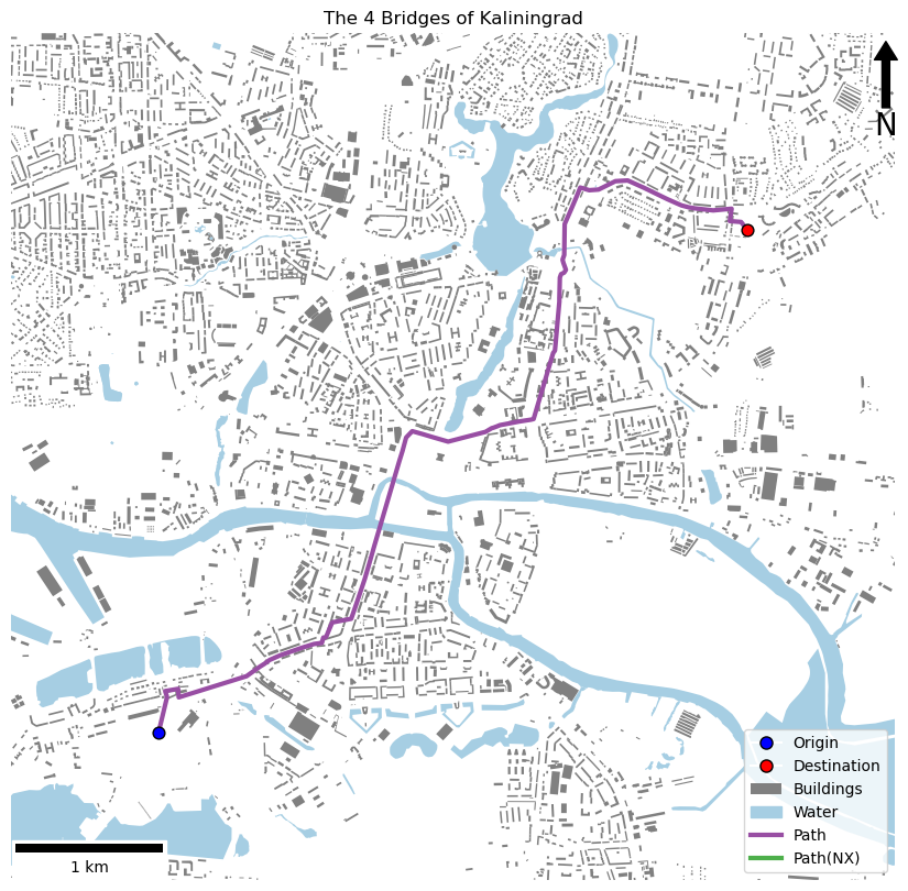
And there you have it, your very own A* Route Planner!

Have a play with the input coordinates and see how many routes you can find. You can use the tool below to get the coordinates of new locations (just click!):

A little more…?

This week has been quite a big practical - but there is plenty more that we can do to hone our skills and improve our route planner:

1. Comparing with networkx

Now that we fully understand the A* algorithm, we have the option of using other implementations (it is perfectly fine to use libraries, providing that you fully understand what they do!). Out of interest, let’s have a look at the implementation of the A* algorithm in networkx:

from networkx import astar_path as astar_path_nx, DiGraph

	# calculate the shortest path using the networkx implementation
	shortest_path_nx = 

Add the above snippets to your code. Note that we are renaming their function as it has the same name as ours!

Complete the second snippet to call astar_path_nx() - click the link and you will see that the arguments for the function are exactly the same as yours. The only difference is that a bug in networkx means that it will not be able to calculate a path on a MultiDiGraph - you will therefore have to convert it to a DiGraph by passing it to the DiGraph() constructor

Pass the resulting path to your path_to_linestring() function, convert it to a GeoSeries, project it and add it to your map so that it appears underneath your original path

Add the below snippet to compare the length of the two routes:

# report the comparative route lengths (using local projection)
print(f"My route: {path.geometry.iloc[0].length:.0f}m. Network X route: {path_nx.geometry.iloc[0].length:.0f}m.")

If all has gone to plan, you should have something like this:

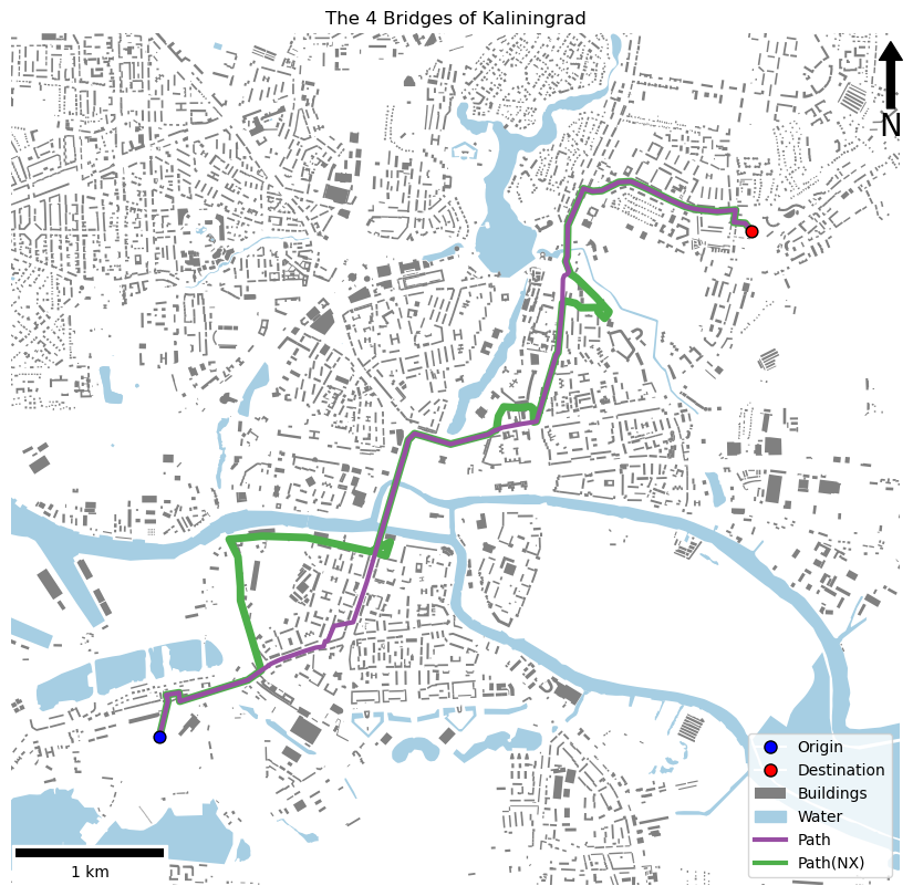
and this:

My route: 6926m. Network X route: 8645m.

That is a difference of >1.5km! Can you think what the differences might be?

2. Serialising data with Pickle

You will notice that it takes quite a long time for this code to run. That is because you are going through the step of importing the OSM data and converting it into a MultiDiGraph every time that it runs, which is quite inefficient (this is also true of loading the two Shapefiles and loading therm into GeoDataFrames)! It would be better if we could import it once, and then save it in a more usable form for future runs.

Fortunately, Python has a function for exactly this, called the Python Pickle. Pickle allows you to serialise a Python object into a file, and then read it in again, which should be much faster than reading data in from other formats. Cases like we have here (where the data are static and take a while to import) are ideal candidates for serialisation with Pickle!

This is another great opportunity to use a try-except statement, which means that we can begin by assuming that our serialised data file is in place, and if it isn’t (which will be signalled by a FileNotFoundError exception), then we can load the data, store the file for next time, and then move on! Here is how:

from pickle import dump, load, HIGHEST_PROTOCOL

# load data from serialised Pickle file
try:
	with open('../data/kaliningrad.pkl', 'rb') as input:
		print("Pickle file found successfully, loading data.")
		
		# extract the serialised MultiDiGraph
		graph = load(input)

# load data from XML and Shapefiles, and create pickle for future use
except FileNotFoundError:
	print("No pickle file found, loading data (takes a long time).")

	# load the MultiDiGraph from the OSM XMl file
	graph = graph_from_xml('../data/kaliningrad/kaliningrad.xml')

	# serialise the dictionary for future use
	with open('../data/kaliningrad.pkl', 'wb') as output:
		dump(data, output, HIGHEST_PROTOCOL)

Can you see how that works? As you can hopefully see, this is quite straightforward - and will make our code much more efficient! The only bit that might not be immediately clear is the HIGHEST_PROTOCOL bit, which is simply describing the method (‘protocol’) by which the data will be encoded. HIGHEST_PROTOCOL makes it use the newest (therefore best, for most purposes) protocol. If you are interested, you can see the options available here.

We could simply repeat this for each of our three datasets, but that would leave us with three files to keep track of. It would be better to load all three of our objects into a single collection (a dictionary in this case) and serialise that using Pickle. Here is how:

from pickle import dump, load, HIGHEST_PROTOCOL

# load data from serialised Pickle file
try:
	with open('../data/kaliningrad.pkl', 'rb') as input:
		print("Pickle file found successfully, loading data.")
		
		# extract the serialised dictionary of the three datasets
		data = load(input)

		# extract the three individual datasets from the dictionary
		graph = data['graph']
		buildings = data['buildings']
		water = data['water']

# load data from XML and Shapefiles, and create pickle for future use
except FileNotFoundError:
	print("No pickle file found, loading data (takes a long time).")

	# load the data from their respective files
	graph = graph_from_xml('../data/kaliningrad/kaliningrad.xml')
	buildings = read_file('../data/kaliningrad/buildings.shp').to_crs(utm34)
	water = read_file('../data/kaliningrad/water.shp').to_crs(utm34)

	# add all three to a dictionary
	data = {
		'graph': graph,
		'buildings': buildings,
		'water': water
	}

	# serialise the dictionary for future use
	with open('../data/kaliningrad.pkl', 'wb') as output:
		dump(data, output, HIGHEST_PROTOCOL)

Edit your code to incorporate the above snippets - remember to remove any other statements that load data, and also that you will probably need to move the definition strings for your CRS’

Now the next time you run your code it will store a pickle file called data.pkl in your data directory. The time after that you run it will use that instead and it will be faster - now you no longer need the .xml or .shp files!