In which we learn how to use genetic algorithms to solve problems for which we don’t even know the solution! It’s practically magic….

Part 1

Introduction to Parallel Computing

Parallel computing is about making use of the features of the Central Processing Unit (CPU) to run code more efficiently. Specifically, we run multiple processes on the CPU at the same time, thus reducing the overall runtime of our code (in comparison with a serial version, in which each task runs one after the other).

Preparing some serial code

There is no better way to understand parallel computing than to give it a go. We will demonstrate parallelisation with a simple example in which we will use our evaluate_distortion() function from week 5 to evaluate the quality of a set of global Equal Area map projections (those recommended by the Projection Wizard) for use in a map of Iceland. As we learned in week 5, Equal Area map projections (particularly global ones) are frequently not as equal area as you would want them to be (see Usery and Seong, 2001, for example) - so this is a worthwile test!

You will hopefully remember that this is a stochastic algorithm, meaning that the randomness in the calculation will lead to small differences between different runs of the same values. As a rule of thumb, the more runs we do, the smaller the variations will be. Unlike last time, when we ran only 1,000 samples per map, this time we will use 10,000. This will give us a much more stable result, but at the cost of around 10x more computing time.

Copy week5.py from the week5 directory into the week11 directory (I know it is not week 11, but we had to move reading week at late notice so the last couple don’t quite align…).

Read the below script and make sure that you understand what it does.

"""
* Script to evaluate which of the Equal Area projections recommended by 
*		projectionwizard.org is the best for use in Iceland
"""
from pandas import DataFrame
from time import perf_counter
from geopandas import read_file
from week5 import evaluate_distortion
from multiprocessing import get_context
from pyproj import Geod, CRS, Transformer

# main code block
if __name__ == "__main__":

    # make a list of dictionaries storing the projections to evaluate
    projections = [
        {'name':'Mollweide', 'proj':'+proj=moll +lon_0=0 +datum=WGS84 +units=m +no_defs'},
        {'name':'Hammer', 'proj':"+proj=hammer +lon_0=0 +datum=WGS84 +units=m +no_defs"},
        {'name':'Equal Earth', 'proj':"+proj=eqearth +lon_0=0 +datum=WGS84 +units=m +no_defs"},
        {'name':'Eckert IV', 'proj':"+proj=eck4 +lon_0=0 +x_0=0 +y_0=0 +datum=WGS84 +units=m +no_defs"},
        {'name':'Wagner IV', 'proj':"+proj=wag4 +lon_0=0 +datum=WGS84 +units=m +no_defs"},
        {'name':'Wagner VII', 'proj':"+proj=wag7 +lon_0=0 +datum=WGS84 +units=m +no_defs"}]

    # set the geographical proj string and ellipsoid (should be the same)
    geo_string = "+proj=longlat +datum=WGS84 +no_defs"
    g = Geod(ellps='WGS84')

    # load the shapefile of countries and extract country of interest
    world = read_file("./data/natural-earth/ne_10m_admin_0_countries.shp")

    # get the country we want to map
    country = world.loc[world.ISO_A3 == "ISL"]

    # get the bounds of the country
    minx, miny, maxx, maxy = country.total_bounds

    # start timer
    start = perf_counter()

    # initialise a PyProj Transformer to transform coordinates
    results = DataFrame(projections)
    for idx, p in results.iterrows():

        # get proj string
        proj_string = p['proj']

        # construct transformer
        transformer = Transformer.from_crs(CRS.from_proj4(geo_string), CRS.from_proj4(proj_string), always_xy=True)

        # calculate the distortion with 10,000 samples
        results.loc[idx, ['Ep', 'Es', 'Ea']] = evaluate_distortion(g, transformer, minx, miny, maxx, maxy, 10000, 1000000, 10000)

    # print the results, sorted by area distortion (drop proj column to make it fit in the console)
    print(DataFrame(results).drop('proj', axis=1).sort_values('Ea'))
    print(f"\nCompleted in {perf_counter() - start:.2f} seconds.")

There should be no surprises there except perhaps for this line:

results.loc[idx, ['Ep', 'Es', 'Ea']] = evaluate_distortion(g, transformer, minx, miny, maxx, maxy, 10000, 1000000, 10000)

which uses .loc to extract the row using its index number (idx) as normal, but then also to select three columns (['Ep', 'Es', 'Ea']) to which the results from our distortion code will be written using variable expansion. This is just a simple way to load data into a dataframe row-by-row. Note that if the columns don’t yet exist (as is the case for the first set of results), .loc will just quietly create the column for us.

Once you understand the code, copy and paste the above code into a new file in your week11 directory called parallel_distortion.py

Run the script

If all has gone to plan, you should get a message like:

          name                                               proj        Ep        Es        Ea
2  Equal Earth  +proj=eqearth +lon_0=0 +datum=WGS84 +units=m +...  0.129131  0.219158  0.000415
1       Hammer  +proj=hammer +lon_0=0 +datum=WGS84 +units=m +n...  0.069124  0.130455  0.002516
5   Wagner VII  +proj=wag7 +lon_0=0 +datum=WGS84 +units=m +no_...  0.102962  0.184200  0.002541
3    Eckert IV  +proj=eck4 +lon_0=0 +x_0=0 +y_0=0 +datum=WGS84...  0.135243  0.228021  0.002547
0    Mollweide  +proj=moll +lon_0=0 +datum=WGS84 +units=m +no_...  0.079358  0.148176  0.002561
4    Wagner IV  +proj=wag4 +lon_0=0 +datum=WGS84 +units=m +no_...  0.104767  0.187198  0.002563

Completed in 4.73 seconds.

You should see that the Ea value is much better for Equal Earth than for the others (but as expected, it does not perform very well in shape and distance as a result).

Note, however, that the reported time will vary between different machines (and even different runs) - this is just one result from my laptop.

Parallelising your code

Whatever amount of time your code took to run, it is probably a fair assumption that it was longer than we would like. We also know that we are not making full use of our CPU, as the whole script is running in serial (i.e., where each projection is evaluated one after the other). This is, therefore, a great opportunity to parallelise our code, so that each projection can be evaluated at the same time. Allowing for some overhead of the parallelisation process (which for small jobs can be greater than the saving…), this should still make our code run much faster than the serial version.

Let’s find out if it does…

Add the following import statement to your code

from concurrent.futures import ProcessPoolExecutor, as_completed

As you can see, we will be using a class called ProcessPoolExecutor to help us parallelise our code. There are multiple ways to do this in Python, but ProcessPoolExecutor from the concurrent.futures is an example of a modern and relatively high-level interface. For those who are interested, an older and lower-level example is available in the multiprocessing library (this is what I actually used in the original GVI calculation).

The first thing that we need to do is identify the part of our code that we want to parallelise and make it into a function. We want to undertake our distortion assessment for each projection in parallel, so we need to move them:

Find these two lines in your code:

# construct transformer
transformer = Transformer.from_crs(CRS.from_proj4(geo_string), CRS.from_proj4(proj_string), always_xy=True)

# calculate the distortion with 10,000 samples
results.loc[idx, ['Ep', 'Es', 'Ea']] =  evaluate_distortion(g, transformer, minx, miny, maxx, maxy, 10000, 1000000, 10000)

Move those two lines into a new function that looks like the snippet below (remember that functions should be above the main code, but below the import statements)

def distortion_worker(geo_string, proj_string, g, minx, miny, maxx, maxy, minr=10000, maxr=1000000, samples=10000):

Change the second line (results.loc…) so that it becomes the return statement for the distortion_worker() function - which should return the Ep, Es, Ea values (rather than writing them into the results DataFrame, as the line previously did)

Each of our processes will call this function at the same time. To allow this to happen, we need to compile the arguments that each process must use when they make their function call. Each one must also reference the index (row number) of the projection in its DataFrame so that we know which process’ results refers to which projection (otherwise they might get mixed up!).

We will refer to this as a list of tasks to be completed (where the evaluation of each projection is one task). I like to compile them as a list of tuples, in which each tuple comprises the index value in position 0 and the dictionary of arguments in position 1.

Create an empty list called tasks immediately above the loop

Now delete the remaining lines of code in your for loop and replace them with this:

# this is a tuple (id, dictionary), where the dictionary is the arguments for distortion_worker
tasks.append((idx, {
    'geo_string': geo_string, 
    'proj_string': p['proj'], 
    'g': g, 
    'minx': minx, 
    'miny': miny, 
    'maxx': maxx, 
    'maxy': maxy
}))

This will populate the tasks list with all of the tasks that

Next (outside the for loop), we use our tasks list to launch our parallel processes. To do this, we simply need to:

1. Create our ProcessPoolExecutor using a with statement to make sure it gets closed properly
2. Loop through tasks, launching a process for each task to call the distortion_worker() function with the specified arguments. This returns an instance of a Future object, which means that it represents something that will happen in the future (i.e., the process completes).
3. Record which Future object is processing which projection using a dictionary called future_map, where the key is the Future object (future) and the value is the index value of the projection in the DataFrame (idx). We can therefore look up the idx value for the projection in any given future simply using future_map[future].

# create an Executor to run GVI calculations in parallel
with ProcessPoolExecutor(mp_context=get_context("spawn")) as executor:

    # submit tasks and keep mapping future -> task idx for assignment
    future_map = {}
    for task in tasks:

        # use variable expansion to get the id of the projection and the function arguments
        idx, args = task

        # submit the task to the executor - this calls the function with the arguments in task_args
        future = executor.submit(distortion_worker, **args)

        # record the ID so that we can assign the correct value later
        future_map[future] = idx

    # report how many processes were launched
    print(f"Launched {len(executor._processes)} processes...")

Note the use of the dictionary expansion operator (**args) - this unpacks the values from the args dictionary and passes every value to the argument with the same name as its key. This is simply a convenience (similar to variable expansion) to avoid us having to do all of that manually.

Read the above carefully and make sure that you understand those three steps

When you do, add the code to your script and run it.

If it has worked, you should get something like:

Launched 6 processes...

The actual number might vary between 1 (the minimum) and 6 (the number of tasks we gave it) depending on the capability of your CPU.

Retrieving your results

Now our processes are all running, we need a way to detect when they finish so we can get the results! For this purpose, we have the as_completed() function, which returns an Iterator over a list of Future Instances that only steps over each one as it completes. This is a very powerful high level tool, as it means that we can simply loop through as_completed(future_map.keys()) ( future_map.keys() gives a list of all of our futures, because we used them as keys in our future_map dictionary), and as_completed() will handle all of the complexity of figuring out when each process has finished!

Our job is therefore to use as_completed() to decide what we want to do when each process finishes - which in our case is simply to load the results into our results DataFrame. Here are the steps:

1. Loop through each Future (one representing each of your processes)
2. Get the index value of the projection it was evaluating using our future_map dictionary
3. Load the resulting values into the relevant columns of our results DataFrame using the same .loc[] statement as before

# process the future objects as they complete using as_completed()
for future in as_completed(future_map.keys()):

    # get the ID for the projection in this process
    idx = future_map[future]

    # get the result for this future object and load into the schools GeoDataFrame
    results.loc[idx, ['Ep', 'Es', 'Ea']] = future.result()

Read the above carefully and make sure that you understand those three steps

When you do, add the above snippet to your code (inside the with block, but outside the for block)

Run the code.

If it has worked, you should now get something like:

          name                                               proj        Ep        Es        Ea
2  Equal Earth  +proj=eqearth +lon_0=0 +datum=WGS84 +units=m +...  0.127806  0.219137  0.000418
1       Hammer  +proj=hammer +lon_0=0 +datum=WGS84 +units=m +n...  0.068642  0.130557  0.002519
5   Wagner VII  +proj=wag7 +lon_0=0 +datum=WGS84 +units=m +no_...  0.102639  0.184265  0.002545
3    Eckert IV  +proj=eck4 +lon_0=0 +x_0=0 +y_0=0 +datum=WGS84...  0.136086  0.227965  0.002549
4    Wagner IV  +proj=wag4 +lon_0=0 +datum=WGS84 +units=m +no_...  0.104069  0.187185  0.002556
0    Mollweide  +proj=moll +lon_0=0 +datum=WGS84 +units=m +no_...  0.079183  0.148175  0.002563

Completed in 1.84 seconds.

As before, the time will be different depending on your system, but it should hopefully be much faster that your previous value!

Part 2

Now we understand the basics of parallel processing, we will apply that knowledge to a more complex situation: calculating the green view index (GVI) (Labib et al., 2021) for 50 schools in a local town called Bolton. I developed GVI with SM Labib (a former PhD student of mine, now an Associate Professor at Utrecht) and Sarah Lindley. This method is now the ‘gold standard’ method for the calculation of visibility exposure.

Because calculating many viewsheds over high-resolution data such as we have here (5m resolution) is computationally intensive, this is a perfect opportunity for parallalisation. When we developed the method, I used parallel code on the University’s High Performance Computing (HPC) facility to calculate GVI for the entirety of Greater Manchester at 5m resolution (>86 million viewsheds), as part of Labib’s PhD studies relating to health and greenspace exposure:

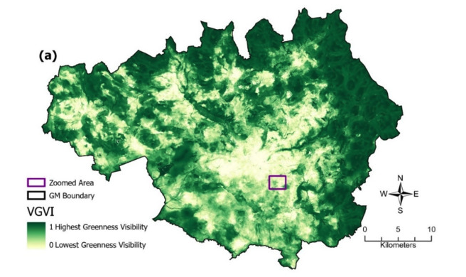
Labib et al. (2021)

We will therefore, have one process to calculate the GVI score for each school. It is unlikely that these will all be able to run at the same time on most machines, and the number that can run at the same time will be dependent on the CPU that you are using, but we should certainly see a big improvement in processing time!

On my machine, this approach uses 10 processes, and processes the 50 schools about twice as fast as the serial version (~25 vs ~50 seconds). This might not seem like quite as good an improvement as you would have expected, but I will explain why this is later in this session.

This is based on a viewshed (as per week 7), so we already have much of the code that we need ready to go:

Read over the below snippet and make sure you understand it - this simply handles imports and functions that we have already understood in previous week 7, so hopefully should be relatively clear.

Note in particular how the line_of_sight_coords() is slightly different from the line_of_sight() function we used in week 7, simply because it returns a list of the indexes (row, col) of the visible cells (rather than updating them directly).

When you understand the snippet below, paste it into your week9/week9.py file

from gc import collect
from math import hypot
from time import perf_counter
from geopandas import read_file
from rasterio import open as rio_open
from rasterio.transform import rowcol
from multiprocessing import get_context
from matplotlib.colors import Normalize
from matplotlib.cm import ScalarMappable
from rasterio.plot import show as rio_show
from matplotlib.pyplot import subplots, savefig
from skimage.draw import line, circle_perimeter
from matplotlib_scalebar.scalebar import ScaleBar
from multiprocessing.shared_memory import SharedMemory
from concurrent.futures import ProcessPoolExecutor, as_completed
from numpy import column_stack, array, dtype, ndarray, nan, intp, sum as np_sum

def coord_2_img(transform, x, y):
    """ 
    * Convert from coordinate space to image space
    """
    r, c = rowcol(transform, x, y)
    return int(r), int(c)


def line_of_sight_coords(r0, c0, z0, r1, c1, radius, dsm_data):
    """
    * Use Bresenham's Line algorithm to calculate a line of sight from one point to another point, 
    *	returning a list of visible cells
    """
    
    # init variable for biggest dydx so far (starts at -infinity)
    max_dydx = -float('inf')
    
    # iterate along integer raster cells on line from observer to target
    visible_coords = []
    for r, c in column_stack(line(r0, c0, r1, c1))[1:]: # skip the observer cell itself
        
        # distance in pixels from observer (Euclidean)
        dx = hypot(c0 - c, r0 - r)

        # if we go too far, or go off the edge of the data, stop looping
        if dx > radius or not (0 <= r < dsm_data.shape[0]) or not (0 <= c < dsm_data.shape[1]):
            break

        # slope from observer to the *top* of this cell
        cur_dydx =  (dsm_data[r, c] - z0) / dx

        # if this slope is greater than any previous slope, this cell is visible
        if cur_dydx > max_dydx:
            visible_coords.append((int(r), int(c)))

            # update max_slope to block further lower-angle points
            max_dydx = cur_dydx

    return visible_coords

Now let’s get some more familiar code out of the way:

Open a main block

Make sure you have the bolton directory located at ../../data/bolton/ - if not, download it here and put it at that location.

Inside it, open two nested with blocks to load ../../data/bolton/bolton_dsm.tif as dsm and ../../data/bolton/bolton_trees_resample.tif as trees

Read the data bands (one each) from those datasets into variables called dsm_data and trees_data respectively

Read the ../../data/bolton/primary_schools.shp into a GeoDataFrame variable called schools

Use .crs.to_epsg() to verify that the epsg code matches for all three layers

Great, now we are set up, we just need our function to calculate GVI function (which is what will be called by the processes). Because this is essentially the same as our viewshed() function, we will move quite quickly over this too:

Take a look at the function in the below snippet.

def gvi_worker(x0, y0, radius_m, observer_height, dsm, trees, transform):
    """
    * Calculate Green Visibility Index based on Labib et al. (2021)
    *   Note that there is no target height in this case, as we are using 
    *   the DSM (so it is 0).
    """

    # convert observer location to raster row/col
    r0, c0 = coord_2_img(transform, x0, y0)
    
    # catch if the dataset is outside the dataset
    if not (0 <= r0 < dsm_data.shape[0]) or not (0 <= c0 < dsm_data.shape[1]):
        print(f"ERROR: data point {x0},{y0} outside of dataset")
        return None

    # radius in pixels (use absolute of pixel x-scale; assumes square pixels)
    radius_px = int(radius_m / abs(transform[0]))

    # observer absolute elevation: DSM value at observer plus observer height
    observer_abs_elev = dsm_data[r0, c0] + observer_height

    # collect visible coords in a set (to avoid duplicates)
    visible = set()

    # add the observer location
    visible.add((int(r0), int(c0)))

    # iterate perimeter points to cast rays
    for rr, cc in column_stack(circle_perimeter(r0, c0, radius_px)):

        # for each line, get visible coords and add to set
        for rc in line_of_sight_coords(r0, c0, observer_abs_elev, int(rr), int(cc), radius_px, dsm_data):
            visible.add(rc)

    # convert to numpy arrays for fast indexing and ensure indices are valid
    rows, cols = zip(*visible)
    rows = array(rows, dtype=intp) # intp is a convenient alias for the default integer type used by the system
    cols = array(cols, dtype=intp)

    # count visible tree pixels
    visible_trees = np_sum(trees_data[rows, cols] == 1)

    # return GVI value (proportion of visible cells that are tree pixels)
    return visible_trees / float(len(rows))

NOTE: Don’t try to run the function at this stage - it needs more work before it is ready to run!

The main bit we need to understand here is the last part…

As with the line_of_sight_coords, this is a slight modification of the viewshed function we used last time. The key difference is that, this time, we are keeping a list of the index (row, col) of each of the visible cells, instead of setting them in an output surface:

# convert to numpy arrays for fast indexing and ensure indices are valid
rows, cols = zip(*visible)
rows = array(rows, dtype=intp) # intp is a convenient alias for the default integer type used by the system
cols = array(cols, dtype=intp)

We then use those indices to see how many of the visible cells also contain trees (by getting the 1 or 0 values from trees_data):

# count visible tree pixels
visible_trees = np_sum(trees_data[rows, cols] == 1)

Finally, we work out the proportion of the viewshed that is taken up by trees (visible_cells / visible_trees) - this is the GVI score!

# return GVI value (proportion of visible cells that are tree pixels)
return visible_trees / float(len(rows))

If the above makes sense, add the gvi_worker() function at the appropriate location in your code (if not, ask!).

Implementing Shared Memory

In our example in Part 1, we did not need our individual processes to have any data resources (e.g., a raster or vector dataset) - as all of the necessary information was included in the function arguments. However, in this case we have several quite large datasets that we need to share.

Unfortunately, we cannot just let multiple processes read and/or write on the same locations in memory (RAM) at the same time, so the Operating System will typically limit them to each have their own process memory space. Because of this restriction, sharing information between processes is difficult and inefficient, normally through sending messages between processes, which normally requires the data to be serialised (converted to binary format), copied, then de-serialised, resulting in a large amount of overhead.

Where multiple processes need to access the same dataset, therefore, our options are essentially:

1. Copy each of the datasets 50 times and pass a different copy to each process (to store in its own process memory space)

2. Use Shared Memory via the multiprocessing.shared_memory library, whereby the data is copied to a new location in memory in which multiple processes are allowed to read and write to the same locations.

With small datasets, option 1 might be possible (noting it will mean the data takes up 50x more RAM!), but it is still highly inefficient (as it still requires the serialise/copy/deserialise process).

Option 2 is therefore preferable in most instances - though it should be noted that it still takes a very large overhead! For context, running this practical in parallel makes it 2x faster on my laptop, but using shared memory and only one process makes it nearly 4x slower - this reveals the extent of the overhead of Shared Memory, and explains why not all tasks are suitable for parallelisation!

The first thing that we need to know about shared memory is that it is quite volatile, and we need to look after it properly (including making sure we remove it when we are done, otherwise it will remain blocked off in RAM!). To do this, it is very important that every process calls the .close() function when it is finished (to close its connection to the shared memory block), and that our software calls the .unlink() function before it finishes (to cleanup the memory block and make it available to the OS again). To be absolutely sure that we have cleaned up properly (which can be a challenge on Windows), we will also use del statements to remove the numpy array instances that reference the shared memory space (dsm_shared_arr and trees_shared_arr), and then force the garbage collector to run (collect()) to clean up any underlying pointers before we try to close() and unlink() our shared memory space.

If either our process or software finishes without calling these functions, then we will lose the reference to the connection / memory block (because they are stored in variables in their respective scope), so we have no way to clean up later. For this reason, we need to take extra care and make sure that they always get called, even if there is an error.

We can do this using a try statement. So far, we have done this in the form of try-except, so ; but as we saw in the lecture, we also have the finally part of the statement available. Let’s revisit how that works:

try:
  # run the code in this block
  
except:
  # if there is an error (Exception) in the try block, run the code in this block instead
  
finally:
  # whatever happens in the above blocks, run this block after they are done

We can therefore use a try-finally block to ensure that, even if there is an error, we will definitely close and unlink our shared data properly. Let’s do it:

Take a look at the statement below, which adds the dsm and trees data into shared memory:

# use try-finally block to ensure that we always close the Shared Memory
try:

    # put DSM in shared memory
    dsm_nbytes = dsm_data.size * dsm_data.dtype.itemsize
    dsm_shm = SharedMemory(create=True, size=dsm_nbytes)
    dsm_shared_arr = ndarray(dsm_data.shape, dtype=dsm_data.dtype, buffer=dsm_shm.buf)
    dsm_shared_arr[:] = dsm_data[:]
    
    ''' ALL CODE USING THE SHARED MEMORY GOES HERE'''

# make sure the below runs, even if there is an error
finally:

    # destroy numpy array object using the shared memory
    del dsm_shared_arr
    del trees_shared_arr

    # now force garbage collection to destroy array base pointers
    collect()

    # finally, it is safe to close and unlink the shared memory
    dsm_shm.close()
    dsm_shm.unlink()
    trees_shm.close()
    trees_shm.unlink()

First, look at the two sections of code in the try block (which create the shared memory objects):

1. First, we need to work out the size of the required block of RAM that needs to be reserved (dsm_nbytes) - this is calculated using dsm_data.size (the number of cells in the raster) multiplied by dsm_data.dtype.itemsize (the size of each cell value in bytes).
2. We then create a shared memory block in RAM (dsm_shm), which is represented by a SharedMemory object - we tell it that we need to create a new memory block (create=True) and the required size of that block (size=dsm_nbytes).
3. Next, we need to create an empty numpy.ndarray (n-dimensional array, dsm_shared_arr) object at the required dimensions (dsm_data.shape) and data type (dtype=dsm_data.dtype) in our shared memory location (buffer=dsm_shm.buf). This is now ready to be populated with values.
4. Finally, we use list slicing [:] to copy all of the data from dsm_data into dsm_shared_arr

Note that this process is not the sort of thing that I would expect you to memorise - but it is something that is important for you to understand.

Once you are satisfied that you understand the above snippet, add it to your main block so that the try block encompasses all of your code that uses the shared memory.

Now, add the necessary code to create a second shared memory block for trees_data (in the try block), then to .close() and .unlink() it (in the finally block).

Attaching gvi_worker() to the shared memory space

Now that is done, we need to make sure that we do the same for any functions that open a connection to the shared memory space. In our case that will be gvi_worker(), which is the function called by each process.

To make this process a little more straightforward, we will make a function to handle it:

Add the below function to your script

def attach_shared_memory(shm_name, shape, dtype_str):
    """
    * Attach to raster dataset in shared memory 
    * Returns: (memory reference, band dataset)
    """
    # get reference to memory location of the shared dataset
    existing_shm = SharedMemory(name=shm_name)
    
    # construct a numpy array object using that location in memory
    shared_data = ndarray(shape, dtype=dtype(dtype_str), buffer=existing_shm.buf)
    
    # return a tuple in the form (memory reference, numpy array)
    return (existing_shm, shared_data)

Now, add the following snippet to the very top of gvi_worker() to connect it to the shared memory space for the DSM dataset:

existing_dsm_shm, dsm_data = attach_shared_memory(*dsm)

Note how two values are returned and stored using variable expansion:

• existing_dsm_shm: an object representing the connection (used to call existing_dsm_shm.close(), for example)
• dsm_data: the values that we stored in the shared memory (the dsm raster surface in this case)

Note also the use of the list expansion operator (*), which is used to unpack the three values that are stored in the dsm tuple (shared_memory_reference, raster_dimensions, data_type) and pass them into attach_shared_memory() in that order, as if they were three separate arguments. As with the dictionary expansion operator (**) that we saw earlier, this is simply for convenience.

Add the equivalent statement to connect gvi_worker() to the trees Shared Memory object

Now, wrap everything in the gvi_worker() function except those two statements in a try block

Then add a finally block at the bottom (after the return statement) and populate it with the necessary code to .close() both shared datasets (but do NOT unlink them as this will delete the shared memory and the other processes will still need it!)

Launching your processes

The rest of the process is effectively the same as it was in Part 1 - we need to make a list of tasks, launch a process for each one, and then get the results using as_completed(). Remember in this coming section that I don’t expect you to have memorised all of this stuff, you can refer to your parallel_distortion.py file for reminders!

Initialise an empty tasks list, then iterate through each school.

Add and complete the below dictionary to the loop in order to populate the tasks list:

# this is a tuple (id, dictionary), where the dictionary reflects the argument for gvi_worker()
tasks.append((idx, {
    'x0': ,	# COMPLETE (x coordinate of origin)
    'y0': ,	# COMPLETE (y coordinate of origin)
    'radius_m': 800,
    'observer_height': 1.7,
    'dsm': (dsm_shm.name, dsm_data.shape, str(dsm_data.dtype)),
    'trees': ,	# COMPLETE  (tuple for info on the trees shared memory object)
    'transform': dsm.transform
}))

Note that we have loaded the raster data bands (e.g., dem_data) into shared memory, not the dataset itself (e.g., dem), so we do not have access to any of the rasterio functionality. For this reason, we are passing the affine transform object (transform) separately so that we can convert between image space and coordinate space when using data in the shared memory space. We are able to only pass one because we know that the rasters are perfectly aligned to each other (i.e., have the same bounds and resolution) - but if this were not the case we would need a separate affine transform object for each dataset.

Add the necessary code to create an instance of a ProcessPoolExecutor (making sure to force the spawn context), then for each task submit a process to run gvi_worker(), remembering to keep track of which Future object corresponds to each school

Add the necessary code to report how many processes you are running

Open a loop using as_completed() to iterate through the Future objects as each process completes.

Inside the loop, open a try block

Inside the try block, load the results into a column called gvi on the correct row of the GeoDataFrame.

Add the except block in the snippet below after it.

except Exception as e:
  print(f"ERROR: Worker raised an exception: {e}")
  schools.loc[idx, "gvi"] = nan

This is handy, as if one of the processes has an exception, then it can tell you that there was a problem, but prevents the exception from killing the whole script (as you have ‘caught’ it), meaning that the script can continue running and you can still see all of the rest of the results, along with the error message.

Finally, add the following (outside the loop!) to report completion:

# report performance counter results 
print(f"{len(schools.index)} Schools analysed in {perf_counter() - start:.2f} seconds.")

Making a Map

Finally, add the below to the bottom of the try block in your main block to plot your results to a map:

# Plot DEM + GVI points
fig, my_ax = subplots(1, 1, figsize=(16, 10))
my_ax.set_title("Green Visibility Index (GVI) per school")

# show trees raster as context (transparent)
rio_show(
    trees,
    ax=my_ax,
    transform = trees.transform,
    cmap = 'Greens',
    alpha=0.4,
)

# Plot schools coloured by computed GVI; use only the selected subset for clarity
schools.plot(
    ax = my_ax,
    column='gvi',
    cmap = 'Greens',
    markersize = 120,
    edgecolor = 'black',
)

# add a colour bar for GVI
if schools["gvi"].notna().any():
    fig.colorbar(
        ScalarMappable(norm=Normalize(vmin=schools["gvi"].min(), vmax=schools["gvi"].max()), cmap='Greens'),
        ax=my_ax,
        pad=0.01,
        label="GVI"
    )

# add north arrow
x, y, arrow_length = 0.97, 0.99, 0.1
my_ax.annotate('N', xy=(x, y), xytext=(x, y-arrow_length),
    arrowprops=dict(facecolor='black', width=5, headwidth=15),
    ha='center', va='center', fontsize=20, xycoords=my_ax.transAxes)

# add scalebar
my_ax.add_artist(ScaleBar(dx=1, units="m", location="lower right"))

# output
savefig('./out/9.png', bbox_inches='tight')

If all has gone to plan, you should now have something like this:

Here, the darker green schools have a view of more trees (with the maximum being ~50% of their total view taken up by trees). Does that meet with your expectations based on the map?

If so then hooray! - you can now do computing in parallel!