In which we learn how to create our own functions, and how to optimise our spatial queries using a spatial index

Getting Ready

Before we start this week, we need to get prepared:

Open up GitHub Desktop and make sure you are logged in and tracking your repository (instructions here if you can’t remember how)

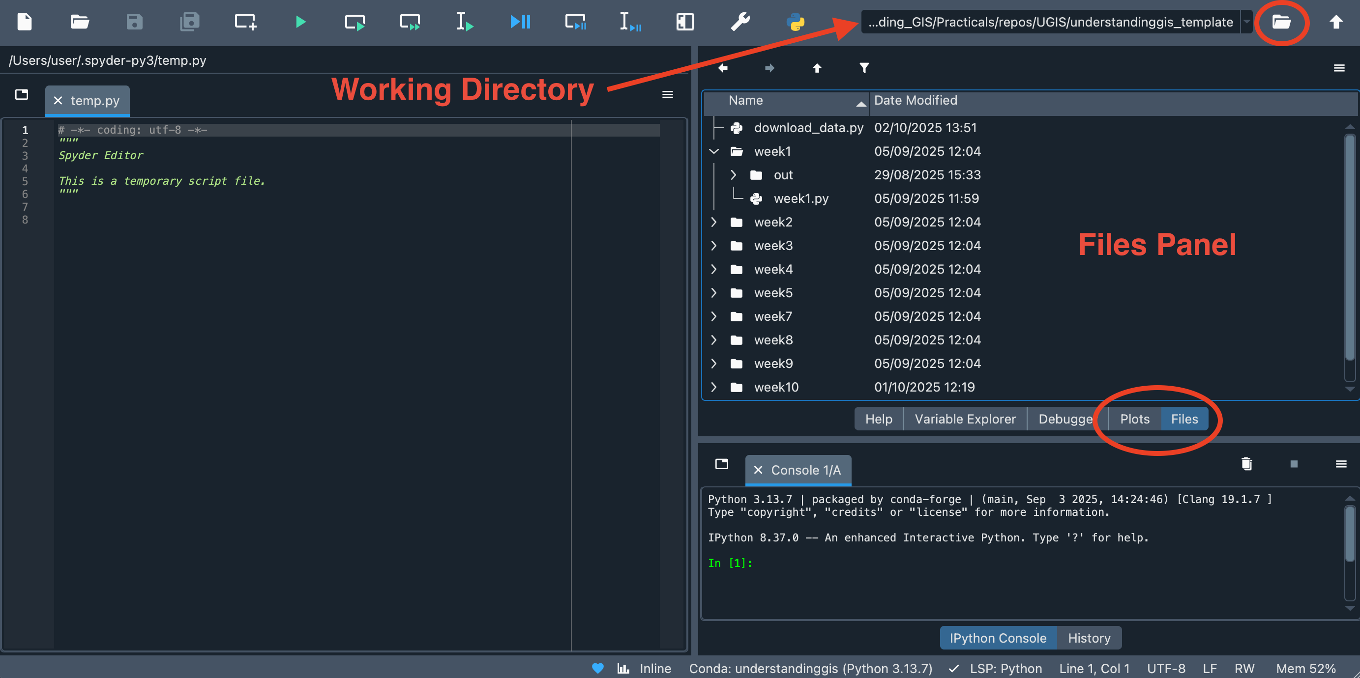
Open Spyder (understandinggis) and make sure that the Working Directory is set to your understandinggis directory. If not, make it so by double clicking on it in the Files Pane or navigating to it using the browse () button in the top right hand corner:

Part 1

Throughout the past two weeks we have made use of several functions in Python (e.g. print(), read_file() g.inv() etc. ). Now we are going to learn to make them for ourselves…

Functions in Python

A Function is simply a bit of code that does something (e.g. print() prints something to the console, read_file() reads a Shapefile into a GeoDataFrame and g.inv() works out the ellipsoidal distance between two locations). Functions are a very useful part of a programmer’s toolkit, as it means that you don’t have to keep repeating yourself in your code - you can simply write a function once and then call it as many times as you like!

In week 2 I told you about a (relatively) simple calculation to get a spherical distance called the spherical cosine method. Below is a Python function that calculates a distance between two points using the spherical cosine method:

Just look at it for now and try to understand it (how the function works, not the maths!). There is no need to do any copying and pasting just yet!

from math import radians, acos, cos, sin

def spherical_distance(x1, y1, x2, y2):
	"""
	This is a special kind of comment used to describe what a function does.
	This one calculates the distance between two locations along a sphere using the Spherical Law of Cosines.
	"""
  # Average radius of WGS84 spherical Earth model in m
  R = 6371008

  # convert to radians
  a = radians(y1)
  b = radians(y2)
  c = radians(x2 - x1)

  # calculate the spherical distance
  distance = acos(sin(a) * sin(b) + cos(a) * cos(b) * cos(c)) * R

  # return the distance
  return distance

Using a function is referred to as calling it. When you call the above function, you pass it some values called arguments (in this case there are 4 arguments: x1, y1, x2, y2). The function processes those values and returns another value (as specified by the return statement in the function definition - in this case, the distance between the two locations described by the four arguments).

To call this function, you would use:

distance = spherical_distance(-2.79, 54.04, -2.75, 54.10)

This will calculate the distance between -2.79, 54.04 and -2.75, 54.10 and store the result in a variable called distance.

Constructing a function

Let’s break that function definition down a little:

Remember - don’t copy and paste anything unless I explicitly tell you to do so!

First, we import some mathematical functions that are required - these come from the math library. This would not normally happen inside the function, but rather at the top of the Python file that contains it (the same place that we always put our import statements!):

from math import radians, acos, cos, sin

Then, we define the function using the keyword def (short for define) - this is where we give it a name and define the list of arguments that it should receive in some parentheses (()). If multiple arguments are required, then we simply separate them by commas (,); if no arguments are required, simply put some empty parentheses (()). Finally, we use a colon (:) to let the python interpreter know that the indented code block that follows is what the function should do (just like in a for loop). As described above, in this case we will use four arguments, describing two coordinate pairs:

def spherical_distance(x1, y1, x2, y2):

The next section should be indented from the definition line (as it is the code block that will run when the function is called - this is just the same as the code block that we used inside our for loops last week). The python interpreter will consider everything that follows the : to be part of the function until it is no longer indented, like this:

def spherical_distance(x1, y1, x2, y2):
	# part of the function...
	# ...still part of the function...
	# ...once again, part of the function...
# ...not part of the function!

You indent things in Python using the Tab button (which might be marked as ⇥ on your keyboard). The indented code block handles the maths to calculate the distance, storing the ultimate result in a variable called distance:

# calculate spherical distance and return
distance = acos(sin(a) * sin(b) + cos(a) * cos(b) * cos(c)) * R

Finally, we return the resulting distance using the return keyword:

# return the distance
return distance

Note that functions do not have to have a return statement. For example, print() is a function that does not return any values (it just prints something to the console), so there will be no return statement in print().

Calling the function

Now that we have a working function, we can call the function to perform a distance calculation. To achieve this, we simply write the name of the function followed by parentheses (()) containing the required arguments (they can be empty if no arguments are required, and they are separated by commas if several are required). If the function returns a value, then we can store that result in a variable using the assignment operator (=) in the normal way:

# calculate the distance between two locations
distance = spherical_distance(-2.79, 54.04, -2.75, 54.10)

# print the value that was returned
print(distance)

The value that was identified by the return keyword is the one that is stored in the distance variable.

Remember that I didn’t ask you to copy and paste any of that, if you did, delete it!

Don’t worry if that seems like a lot to take in, once you start writing functions for real it will all become perfectly clear! Let’s get started right now…

Open week3/week3.py and create a function for measuring distance using the Pythagorean Theorem, based upon the below template - functions should be located at the top of your code, but below any import statements. You will need this in Part 2 so make sure you keep a copy of it!

# THIS IMPORTS A SQUARE ROOT FUNCTION, WHICH IS A BIG HINT!!
from math import sqrt

def distance(x1, y1, x2, y2):
	"""
	* Use Pythagoras' theorem to measure the distance. This is acceptable in this case because:
	*	 - the CRS of the data is a local projection
	*	 - the distances are short
	*  - computational efficiency is important (as we are making many measurements)
	"""
	return # complete this line to return the distance between (x1,y1) and (x2,y2)

Hint: if you get stuck, remember that the material from Week 2 might help you out!

Warning: When running copied and pasted code, you might get an error that looks like this:

 unindent does not match any outer indentation level

This means that the indentations in your code are a mixture of spaces and tabs, which is confusing the Python interpreter. Fortunately, this is an easy fix - you can either:

• Get Spyder to do it for you by selecting Source → Fix Indentation
• Manually replace the offending space-based indents with tabs (just delete the indentation, and then tab the line back across to where it is supposed to be). Remember that the error message will tell you which line is causing the problem, and that you might have to replace a few lines before it starts working (normally all of the lines that you just pasted).

Either way should work fine! Be sure to remember this - it will come up relatively often during your Python career - it is the price we pay for the simple indent-based syntax (and also for copy-pasting code from the web…)!

Test your function to get the coordinates between 345678, 456789 and 445678, 556789 to make sure that it works correctly

You should get something like the following result:

141421.35

If so, then great! Your function works!!

It’s not time to commit your changes to Git. As tyhis is our first week using GitHub Desktop, here is a reminder of what to do:

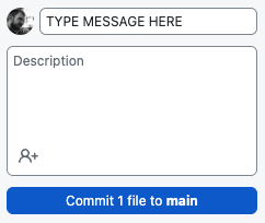
Here is how to use it:

• When you are ready to commit, simply add a short message to the Summary box (ignore the Description) and click the blue Commit to main button.

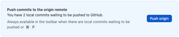
• When you are ready to push (I would just do this every time you commit), either click the blue Push origin button that appears in the panel on the right (which will only be there just after you commit), or the Push origin button in the black bar at the top (which is always there).

OR

Got that? Let’s do it…

And now, back to the lecture…

Part 2

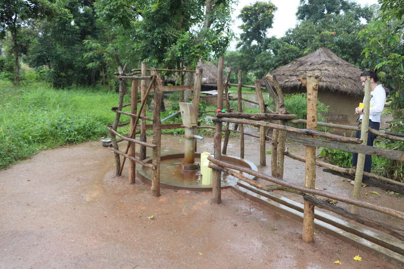
This week we are going to have a look at a part of my research, which looks into the optimisation of borehole locations (for drinking water) in Northern Uganda in order to reduce inequalities in access to clean water. This is a borehole (with one of my former PhD students hiding behind a stick…):

We are going to undertake one part of the analysis involved in this work, which is to calculate the mean distance that anyone has to walk to get to the nearest borehole within their district. This is important because water supply in Uganda is managed at district level, and so the analyses need to reflect this.

As map data are scarce in this region, we will do this making some assumptions and accepting some caveats:

• in the absence of a complete network dataset, distances will be measured ‘as the crow flies’. This is not an unreasonable assumption here because:
  • the distances are generally quite so small the difference will generally also be quite small
  • many people do not travel along the network, but will go through fields etc to collect water. For this reason, a network distance can actually overestimate distances
• people’s location will be calculated using a population data model made available by Facebook Labs. This is probably the best available population data for this region, but is certainly not perfect.
• existing borehole locations will be taken from a dataset made available by the Ugandan Bureau of Statistics. We know that this is incomplete, but it is (again) the best available. This dataset covers a much larger area, and so will need to be cut down to the district first.

Following our discussion in the lecture, we know that there are several ways that we could approach this task, but the volume of data that we are dealing with dictates that we should make use of a spatial index in order to make our calculations as efficient as possible.

In order to aid our understanding, we will begin by making our own spatial index using the STRtree class in the shapely library. This is an implementation of the RTree algorithm that we discussed in the lecture Guttman, 1984, but it uses a faster approach to loading the bounding boxes into the RTree that was developed by Leutenegger et al., (1997).

Before we move on to spatial index, though, we need to take a moment to consider our data…

Matching up the CRS’

Before we embark on any GIS analysis, we must always take time to consider the CRS. This is especially important in this case, because we are going to be making our distance calculations using projected coordinates. Distortions in the projection will therefore significantly affect our results if we are not careful. We therefore need to make sure that all of our datasets are using the same CRS, and that the CRS is appropriate for our area of interest (Northern Uganda).

Before we do anything - we should really have a look at what CRS’ the datasets are already using. Fortunately, geopandas makes this very easy for us. As we already know, when we open a dataset using read_file(), we get a GeoDataFrame object back, which includes a set of properties and functions. Amongst these are everything that we need to check the CRS of our dataset (with the .crs property) and change the CRS of the dataset (with the .to_crs() function).

Firstly, let’s take a look at our data, add the below snippets to your code to load the three datasets (below, but outside the distance() function that you made in part 1):

from geopandas import read_file

# read in shapefiles, ensure that they all have the same CRS
pop_points = read_file("../../data/gulu/pop_points.shp")
water_points = read_file("../../data/gulu/water_points.shp")
gulu_district = read_file("../../data/gulu/district.shp")

NOTE: If you have a file not found error - you can solve this by proactively correcting the path. Your working directory (i.e., the start point) is in the top right in Spyder, and should end with either understandinggis or week3 - given you know that ../ means “go up a level”, it should be relatively straightforward for you to correct the file path and resolve the error yourself.

As we discussed in the lecture, there are three main ways to represent CRS’:

• EPSG Codes (an ID number allocated by the European Petroleum Survey Group)
• Proj Strings (a short formatted String of text defined by the developers of the Proj library)
• WKT Strings (a long formatted string defined by the Open Geospatial Consortium)

The difficulty is that if we were to print use the .crs property, it could come out using any of these three definitions (and could vary between datasets too), which can make them very hard to compare. Fortunately, we can specify which form we would like our output to be in using these member functions of the CRS object that is returned by .crs:

• .to_epsg() - represent the CRS as an EPSG code
• .to_proj4() - represent the CRS as a Proj String
• .to_wkt(): represent the CRS as a WKT String

Because they are member functions of the CRS object, you use them by simply appending the .to_epsg() function to the .crs in each of your statement (as .crs is a property of the GeoDataFrame Object that provides an Instance of a CRS Object that represents the CRS of your GeoDataFrame). For example, to get a proj string for the pop_points layer, you would use pop_points.crs.to_proj4().

Use .to_epsg() to print() the EPSG code for each of your datasets

If it went to plan - it should look like this:

21096

4326

21096

Examining the CRS of pop_points and gulu_district:

Now we have our EPSG codes, let’s see what they all mean: You can look up pre-existing projections by their code in the EPSG database using websites such as epsg.io. You can simply type in the number and it will show you the details of the corresponding CRS:

Find the details for the CRS with the EPSG code 21096

If all has gone to plan, you should be looking at the details of a CRS called Arc 1960 / UTM zone 36N. This is part of the Universal Transverse Mercator (UTM) system, in which the majority of the surface of the Earth is divided up into 1,144 zones that are (mostly) in a 60 × 20 grid of local projections designated by a code in the order column, row, where the column is a number between 1 and 60 and the row is a letter between C and X. Here are the zones that cover Africa (click here to see the full grid):

Source, Wikipedia

As you can see, your projection is UTM zone 36N, which you can confirm covers Northern Uganda in the above image. We are lucky that our area of interest falls entirely within one UTM zone - as you can see, they rarely align with countries. As we saw in the lecture, UTM zone 36N is a local conformal projection that is quite similar to what we might have made using the Projection Wizard.

Note also that the full name of this projection is Arc 1960 / UTM zone 36N. The Arc 1960 part refers to the datum that the CRS uses (this is the reference frame that maps an ellipsoid to the Earth - in this case, the ellipsoid is Clark 1880). Like the projections that are built on top of them, datums also have local and global variants. You will remember that we have so far used the WGS84 datum, which is a global datum, meaning that it is generally a good fit for the geoid at a global scale. However, for work in a specific location, a local datum is generally a better fit at that location (but will be worse elsewhere). In the case of Africa, the Arc 1960 local datum is therefore a better choice, as it was designed specifically for use in Africa.

For reference, if you scroll down a little on the epsg.io page, you will see a variety of ways that you can export your the projection, including Proj Strings (listed as Proj.4, an old name for the Proj software) and WKT Strings (listed as OGC WKT). In this case, we do not need them, as we already have the CRS stored in our pop_points object!

Matching up the CRS’ of our datasets:

We can plainly see that these datasets are all stored using different CRS’. This is a critical issue for analysis as the datasets will be misaligned if they are not in the same CRS. We therefore want to make it so that they all match up, which we can do using the .to_crs() function of the GeoDataFrame object. Here is an example:

# read in the `water_points` dataset AND transform it the the same CRS as `pop_points`
water_points = read_file("../../data/gulu/water_points.shp").to_crs(pop_points.crs)

Based on the above example, ensure that all of your layers to the Arc 1960 / UTM zone 36N CRS - note that you can edit your existing lines of code by adding .to_crs(pop_points.crs) to the end of your existing lines of code (you don’t want to open a second copy of the dataset!!)

Check that this has worked by printing the CRS of all three again. They should all now be the same!

Once you are satisfied, comment out all of your print() statements relating to CRS’

Building a Spatial Index

A Quick note on Spatial Indexes and GeoPandas

As we know, geopandas is a very high-level library that is aimed at Data Scientists, and as such it has a tendency to mask much of the computational work that goes on in the background, which is directly at odds with the purpose of this course! Spatial index functionality is one such example, as geopandas will automatically use a spatial index for you in order to help with some topological operations on GeoDataFrame / GeoSeries objects.

Whilst this is convenient for a general geopandas user, it is not a great way to understand what a spatial index is, nor how one is used; which is the main purpose of this course. For this reason, we will first create our own spatial index to help us understand it, before converting our code to the higher-level geopandas version for comparison, which will nevertheless be useful in your day-to day coding practice.

It is worthy of note that later in the course we will need to build spatial indexes for datasets that cannot be stored in a GeoDataFrame, so understanding how to do it for yourself is essential, even if you would normally prefer to rely on geopandas to do it for you!

For reference, it is also worth noting that there are other options available to you for spatial index libraries, including rtree, which uses the traditional RTree algorithm (which is a little slower than STRTree, but allows editing once it has been created, which shapely.STRtree does not), and scipy.spatial.KDTree, which uses a different underlying algorithm (similar to one we explore in Week 9). Both are also available in the understandinggis environment.

Building your own Spatial Index with shapely.STRtree

Now we are happy that our data is ready for use, we can make a start with our analysis.

The first thing that we need to do is to remove all of the points from water points that are outside of our area of interest (which is defined by Gulu District). This should be simple enough based upon our knowledge of Topology from last week: we simply need to extract all of the points that are within the district polygon, and discard the rest.

Once we have done that, our second job will be to work out the nearest feature in well_points (borehole) to each feature in pop_points (house) and calculate the distance between them using the distance() function that we created earlier. We can then map those differences and see what patterns emerge!

Both of these sound quite simple on the face of it, and they are. The problem only arises from the volume of data with which we are dealing:

Add the below snippet to your code to see how many wells and population points we have:

print(f"population points: {len(pop_points.index)}")
print(f"Initial wells: {len(water_points.index)}")

Note the form f"...". You have seen statements like this before in this course - they are called f-strings (which means formatted string literals), and are a simple way to combine python functions with text output. You simply add an f to the start of the string definition, and then you can put Python statements inside curly braces { } inside the string. At the time that the string is used, the python values are calculated, and the results are added into the string - Simple! You can read more about f-Strings here.

Note also the form of the statement {len(pop_points.index), which is used to calculate the number of rows in a geodataframe to Python’s built-in len() . It is important to note that you must pass .index or a column of a geodataframe to the len() function if you want to get the number of rows - if you pass the geodataframe itself then it will give you the number of columns, which can be very misleading!

If you run the above print() statements, you should see that we have 3,000 boreholes and over 42,702 population points - that would mean we need over 128 million distance calculations…! Whilst this is certainly possible, it would be extremely inefficient and will take a very long time. The solution, as we saw in the lecture, is to use a Spatial Index in order to reduce the number of calculations that we need to do to answer this questions, and therefore make our program much more efficient.

As described above, we will do this first using the STRtree class of the shapely library, which implements the approach suggested by Leutenegger et al., (1997). This is faster than the original specified by Guttman, (1984), but once created it is read only, meaning that no further objects can be added or removed from the index without a complete re-build. This is a common theme in spatial index software, which often includes versions that are faster, but read only; or slower and editable.

Look carefully at these two snippets and the paragraph below it, making sure that you understand them

from shapely import STRtree

# get the geometries from the water points geodataframe as a list
geoms = water_points.geometry.to_list()

# initialise an instance of an STRtree using the geometries
idx = STRtree(geoms)

This short statement simply extracts all of the geometries from the water points geodataframe, converts it from a pandas.Series object to a list (with .to_list()) and then loads it into a STRtree() object. The STRtree constructor will then calculate the bounding box (the smallest rectangle aligned to the axes of the CRS that contain the feature) for each geometry and load it into the RTree spatial index.

Add the above two snippets to your code at the appropriate locations in order to construct a spatial index on the water_points dataset using shapely.STRtree:

At this point, we have a working spatial index - hurrah!

Optimising Intersections with a Spatial Index

Now we have our spatial index, we can put it to work by making it help us to filter our wells dataset to exclude all boreholes that are outside of the Gulu District (which is defined by the polygon stored in district).

This is how the process will work:

1. Get our spatial index representing boreholes
2. Use it to very quickly return the index (ID) numbers of all of the boreholes that are contained within the bounding box of district
3. Query the GeoDataFrame (using .iloc) to return the rows that match that list of index (ID) numbers
4. Use a topological within test to assess whether each geometry in the resulting (much smaller) dataset is inside the district or not.
5. Re-build your spatial index to only include those features that are within the district polygon.

The result of this approach is that we only need to do a within query on 1,002 geometries, rather than the full 3,000, meaning that the operation will only take about a third of the time to run. Pretty good eh!

Let’s give it a go:

Paste the below four snippets into your code to utilise the spatial index, making sure that you fully understand each step:

1: Retrieve the polygon geometry using .iloc[0] (i.e., get the dataset at index location 0 - this is the first, and in this case only, row in the table) and report the number of boreholes in the dataset using a print() statement and f-string.

# get the one and only polygon from the district dataset
polygon = gulu_district.geometry.iloc[0]

# how many rows are we starting with?
print(f"Initial wells: {len(water_points.index)}")

2: Use the .query() function of your STRtree object to return a list of the ID’s of the boreholes that intersect the bounds of the district polygon. Note that this is simply a list of the ID’s, not the features themselves!

# get the indexes of wells that intersect bounds of the district
possible_matches_index = idx.query(polygon)

3: Use the resulting list to query the water_points GeoDataFrame using .iloc (notice that this time we are passing a list of index numbers to it, rather than just a single one as in step 1). Report the number of boreholes that meet this criteria.

# use those indexes to extract the possible matches from the GeoDataFrame
possible_matches = water_points.iloc[possible_matches_index]

# how many rows are left now? 
print(f"Filtered wells: {len(possible_matches.index)}")

Note that we work this out by printing the length of one column. In this case, we are using the index, which is the list of ID numbers that correspond to each row (0, 1, 2, etc.). Though any column would do, we normally use index as this is the column that is guaranteed to be in every single dataset!

4: Finally, use the smaller dataset to do the (slower but more precise) within query. This time, instead of a list of ID numbers ([1, 5, 17, etc...]) we get a list of Boolean values back ([True, False, True, True, etc...]), with one value for each row describing whether or not it is within the polygon or not. To extract the corresponding rows this time, we must therefore use .loc (which can take a Boolean input), rather than .iloc (which only takes a list of index numbers):

# then search the possible matches for precise matches using the slower but more precise method
precise_matches = possible_matches.loc[possible_matches.within(polygon)]

# how many rows are left now?
print(f"Filtered wells: {len(precise_matches.index)}")

Once you are sure you understand the above steps, run your code

If all has gone to plan, you should now have a list of 744 boreholes in the Gulu District of Northern Uganda:

Initial wells: 3000
Potential wells: 1002
Filtered wells: 744

Optimising Nearest Neighbour with a Spatial Index

Now we have filtered our borehole dataset, it is time to do our actual analysis. To do this, we need to know the distance from each population point to its nearest borehole. Once we know this, we can easily work out the mean distance. We could do this by working out the distance from each population point to each borehole, and then take the minimum for each one. The downside is that this would be (42,702 × 744 =) 31,770,288 distance calculations, which would take quite a while!

Fortunately, we can reduce this substantially by once again leveraging the power of our Spatial Index. In this case, we are going to use the idx.nearest() function in order to determine the nearest neighbour of each of our population points, reducing the number of calculations from nearly 32 million to just 42 thousand. This is another huge gain in efficiency, as it avoids ~99.9% of the computation that we would otherwise have had to do!

Rebuilding out Spatial Index

However, before we can do anything with our Spatial Index, we need to stop and think for a second… We are now in the position where we have reduced the amount of data in our GeoDataFrame (now only 744 boreholes), but our Spatial Index no longer matches it (as it still contains 3,000 boreholes).

If we had completed our analysis and were not planning to make any more use of the Spatial Index, then this would be no problem, but in our case we are going to use it again, so we need to re-build it to make sure that it matches the GeoDataFrame. As we know that a shapely.STRtree object is read only, our only option is to simply re-build the index from scratch. To do this, we will overwrite the idx variable with a new STRtree object that reflects the contents of precise_matches instead of water_points.

Paste in the below snippet and add the missing lines to rebuild the index to only include the boreholes in precise_matches (this is just the same as you did before, except with a different geodataframe):

# rebuild the spatial index using the new, smaller dataset
idx = 

Nearest Neighbour analysis with STRtree (and iterating through a geodataframe)

To undertake the next part of the analysis, we want to loop through each population point, calculate the nearest water point (using our Spatial Index for speed), and determine the distance to it. However - we need to think carefully for this step, as looping (or iterating) through a geodataframe is not quite as straightforward as we would like it to be… Here is how it is done:

# loop through a geodataframe called gdf
for id, row in gdf.iterrows():
  
  # here row contains a single row of data
  print(id)						# print the index value (normally the row number) of the current row
  print(row.geometry)	# print out the geometry in the current row
  print(row.name)			# print the contents of a column called 'name'
  print(row['name'])	# alternative way to print the contents of a column called 'name'

An irritating feature of the GeoDataFrame data format, is that you cannot simply loop through the rows contained within it using a statement like for row in gdf:. Doing this will return valid code, but it will loop through the column names of the GeoDataFrame, not the rows of data. This is the reason why len(gdf) returns the number of columns, not the number of rows, so we have to use len(gdf.index) instead.

If you want to loop through the rows of data in a GeoDataFrame, you have to use its .iterrows() function to return an Iterable representation of the data rows, and then loop through that. Here is how it works:

# loop through each population point
for id, house in pop_points.iterrows():

As you can see, .iterrows() returns two values in each iteration of the loop (as opposed to the one value that we were getting last week). For this reason, we have two variables in our for statement: id and well (remember that these are variables so you can call them whatever you like):

• id contains the index of the dataset - this is a unique identifier for each line, and by default will simply be a series of numbers (0, 1, 2, 3 etc…). This is the number that .iloc (index location) was using last week.
• well contains the actual row of data in the loop, giving you access to all of the columns including the geometry.

This is really important, as lots of errors in pandas and geopandas scripts occur as a result of people forgetting to use len(gdf.index) when calculate the number of rows, and gdf.iterrows() when iterating through the rows!

Make sure that this makes sense to you. If you don’t get it - ask!

Now we understand that, let’s get stuck in to out analysis:

Declare an empty list in a variable called distances (If you can’t remember what to do, you can use the hints page to find information on defining an empty list)

Open a for loop that iterates through the pop_points dataset, using the variables id and house to store the index and row respectively

Once you have done that, it is time to put a block of code inside your loop. We have three steps to complete for each population point:

1. Get the index of the nearest well to the current population point (house), extract the one and only value from the list
2. Use the resulting index number to get the relevant row using .iloc
3. Measure the distance between the current population point and the nearest borehole, append the result to the distances list that you initialised outside of the loop

Here’s how:

1: Get the index of the nearest well to the current population point using the .nearest() function of your STRtree object (stored in the idx variable):

# use the spatial index to get the index of the closest well
nearest_well_index = idx.nearest(house.geometry)

Add the above snippet to your loop (pay attention to the indentation to make sure that it is inside the loop block!)

2: As with query(), the spatial index only gives us a list of the ID of the nearest borehole, not the row from the water_points dataset itself. Once again, we therefore need to get the corresponding row of data from the GeoDataFrame using your index and .iloc

	# use the spatial index to get the closest well object from the original dataset
	nearest_well = 

Add and complete the above snippet to your loop block to extract the row of data corresponding to the nearest well from precise_matches using .iloc, then use .geometry to get the geometry itself.

3: Irritatingly, the wells are being returned as a MultiPoint, rather than a Point object in this case (you could verify this with print(type(nearest_well)) if you wanted). A MultiPoint is simply a collection of individual Point objects (a list containing only one element in this case). It is a little unusual in this case because there is only one Point in the MultiPoint, but this is a genuine artefact of this dataset, and so I have left it in as an illustration of the sort of unexpected challenge we need to be prepared to deal with when using real datasets.

All we need to do is extract the Point object from the MultiPoint. To do this, we use the .geoms property to return all of the Points in the MultiPoint as a list (though again, there is only one Point in the list) - note that this same property also works for MultiLineStrings and MultiPolygons - and then extract the first element from the list with [0]:

.geoms[0]

Append the above snippet to the end of the line beginning nearest_well = ... to extract the individual Point from the MultiPoint object.

4: Finally, measure the distance using your distance() function from Part 1 and append the result to your distances list using distances.append():

# store the distance to the nearest well
distances.append(distance(house.geometry.x, house.geometry.y, nearest_well.x, nearest_well.y))

Note that these steps could be done across two separate lines of code (first get distance, then add to the list), but as we will not use the distance value for anything else, this is a more elegant solution (as it avoids the unnecessary creation of a variable).

Add the above snippet to the loop (pay attention to the indentation!)

Add a temporary print statement to check the length of the distances list and run your code to make sure that it all works.

Look back over the code that you have so far and make sure that you understand how it works.

A note on the Distance Function

In contrast to last week, where we were measuring a single, very long distance; this week we are measuring lots of very short distances. In order to enable us to do this efficiently, we decided not to use the most precise measurement technique (the inverse Vincenty method), but rather use the much more efficient approach of using the Pythagorean Theorem (measuring on a flat surface), which is less computationally intensive. This is particularly the case with data that are already projected, such as this one, as we would need to first de-project the data to 3-dimensional longitude-latitude coordinates before we could calculate the ellipsoidal distance!

We can get away with this because we have selected an appropriate local projection (which minimises distortion) and are measuring over sufficiently small distances (mostly <1km). The combination of these facts means that we can be confident that any error will be negligible.

Also note that there are .distance() functions available in shapely and geopandas, which you may prefer to use in future code that you write. However, as with the spatial index, it better suits the goals of this course (to understand what is happening, not simply how to make it happen) to use a distance function that you have created yourself. It is a common mistake for people to inappropriately use built-in functions such as .distance() , without considering the implications for the accuracy of their measurement (see last week).

Using our Distance Data

If all has gone to plan, you should now have a list of 42,702 distances (in metres), and have verified this using your print() statement. It doesn’t run instantly (we are still doing a lot of work here), but shouldn’t take too long.

We should also check the contents of the list, but clearly we don’t want to print such a large number of values to the console. A good compromise is just to print a small number. For example, you could print the first 5 entries like this:

print(distances[:5])

This technique is called list slicing - and simply means print from the start of the list (:) to the fifth item (5) only. We will return to list slicing in more detail later in the course.

Try the above snippet to see if your distance data are as expected

Now we have a list of distances, we can add them to our pop_points dataset as a column - where each row in the column represents the distance to the nearest well for that house (in metres). We saw how to do this in week1, it is very simple:

# store distance to nearest well
pop_points['nearest_well'] = distances

Add the above snippet to your code and run it - then test if it works by printing the columns list for this dataset.

We can also use our list of distances calculate the mean distance, which is simply a matter of dividing the sum of all of the distances (sum(distances)) by the number of distances (len(distances)) - both sum() and len() are built in functions, and so do not need to be imported.

Calculate the mean distance and store it in a variable called mean

Now, we can report some simple statistics about the distances using f-strings:

print(f"Minimum distance to water in Gulu District: {min(distances):,.0f}m.")
print(f"Mean distance to water in Gulu District: {mean:,.0f}m.")
print(f"Maximum distance to water in Gulu District: {max(distances):,.0f}m.")

Add the above snippet to your code and run it

If all has gone to plan, you should have something like the following:

Minimum distance to water in Gulu District: 1.6317053838969449m.
Mean distance to water in Gulu District: 863.0781936686474m.
Maximum distance to water in Gulu District: 10386.960935813864m.

This is all well and good, but isn’t a very good way to present the numbers - there are far too many decimal places, giving an unrealistic impression of precision. We can replace this by specifying some modifiers for our f-strings:

print(f"Minimum distance to water in Gulu District: {min(distances):,.0f}m.")
print(f"Mean distance to water in Gulu District: {mean:,.0f}m.")
print(f"Maximum distance to water in Gulu District: {max(distances):,.0f}m.")

Note how we added :,.0f to the end of the number in the f-strings here. This is a modifier, which is used to set how you would like the number to be displayed. Let’s look at the components more carefully:

• : is used to denote the beginning of a modifier
• , is used to use the , character as a thousands separator
• .0f is used to represent it as a fixed point number with 0 decimal places (i.e., an integer). .2f, for example, would then give two decimal places, and so on

A full list of the available modifiers is provided here (but you’ll need to scroll down to it).

Replace your print statements with the above snippet and run the code again

If all has gone to plan, you should now have something like the following:

Minimum distance to water in Gulu District: 2m.
Mean distance to water in Gulu District: 863m.
Maximum distance to water in Gulu District: 10,387m.

Much better!

If so then well done - your analysis is complete! Now we just need to plot a map…

Plotting the Map

Plotting this map is nothing that you haven’t seen before in weeks 1 and 2, but be sure to have a read through and make sure that you understand it - as you will have to be able to plot maps on your own soon:

from matplotlib_scalebar.scalebar import ScaleBar
from matplotlib.pyplot import subplots, savefig, title

# create map axis object
fig, my_ax = subplots(1, 1, figsize=(16, 10))

# remove axes
my_ax.axis('off')

# add title
title("Distance to Nearest Well, Gulu District, Uganda")

# add the district boundary
gulu_district.plot(
    ax = my_ax,
    color = (0, 0, 0, 0),	# this is (red, green, blue, alpha) and means black, but transparent (alpha=0)
    linewidth = 1,
	edgecolor = 'black',		# this is just a shortcut for (0, 0, 0, 1)
    )

# plot the locations, coloured by distance to water
pop_points.plot(
    ax = my_ax,
    column = 'nearest_well',
    linewidth = 0,
	markersize = 1,
    cmap = 'RdYlBu_r',
    scheme = 'quantiles',
    legend = 'True',
    legend_kwds = {
        'loc': 'lower right',
        'title': 'Distance to Nearest Well'
        }
    )

# add north arrow
x, y, arrow_length = 0.98, 0.99, 0.1
my_ax.annotate('N', xy=(x, y), xytext=(x, y-arrow_length),
	arrowprops=dict(facecolor='black', width=5, headwidth=15),
	ha='center', va='center', fontsize=20, xycoords=my_ax.transAxes)

# add scalebar
my_ax.add_artist(ScaleBar(dx=1, units="m", location="lower left", length_fraction=0.25))

# save the result
savefig('out/3.png', bbox_inches='tight')
print("done!")

Make sure that you understand the above two snippets. If so, add them to your script and run it. If not, ask!

If all has gone to plan, you should have something like this:

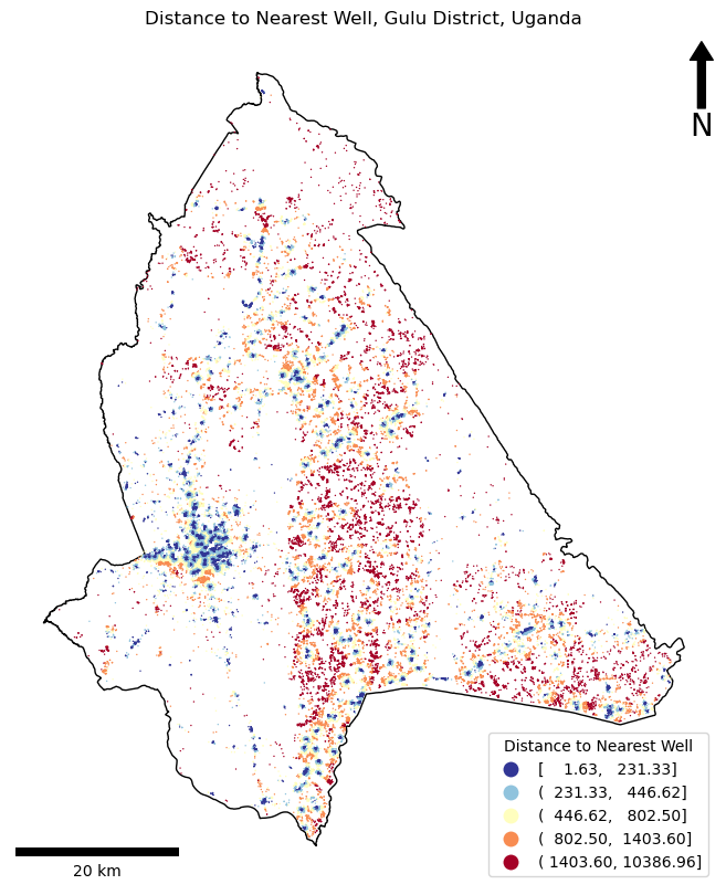
If so, Congratulations!! There are some very clear spatial patterns here that we could now further analyse in order to quantify the apparent patterns in the inequality of access to water.

One thing to pay attention to is the legend - the automated classification has surrounded the numbers with a mix of brackets (various combinations of () and []). Though some people think that this looks untidy - this is actually scientific notation for ranges:

• [a, b] means that the range is inclusive - it includes the values a and b.
• (a, b) means that the range is exclusive - it does not include the values a and b.

From there you can start to mix and match. For example, (a, b] therefore means that the range includes all values greater than a (>a) and less than or equal to b (<=b). Simple!

Finally, demonstrate your understanding by having a play with different classification schemes and colour ramps.

Once you are happy that you understand how this all works, you’re done! This was a challenging week, so very well done and I’ll see you next week!

A little more…?

If you still have the energy - here are a few more things for you to think about:

Considering edge cases

Adjust your analysis so that it includes water points that are within 10.5km of the border of Gulu District

This is important, as the nearest water source for some people might actually be outside of the area! This is, after all, nothing more than an arbitrary political boundary - it will have little or no bearing on people’s behaviour. By limiting it to 10.5km (roughly the maximum distance anyone has to travel in the current model), we can still keep our analysis efficient, whilst ensuring that any relevant wells are included.

To achieve this - we simply need to buffer the geometry of the District (stored in polygon) by 10,500m. This can be achieved using the .buffer() function included in Shapely (and so available on the geometry object that you extract from geopandas):

You will notice that this increases the number of wells in the analysis, but (in this case) only makes a very small difference to the mean result (it does not affect the maximum or minimum distance):

Before:

Initial wells: 3000
Potential wells: 1458
Filtered wells: 975
Minimum distance to water in Gulu District: 2m.
Mean distance to water in Gulu District: 864m.
Maximum distance to water in Gulu District: 10,387m.

After:

Initial wells: 3000
Potential wells: 1458
Filtered wells: 975
Minimum distance to water in Gulu District: 2m.
Mean distance to water in Gulu District: 863m.
Maximum distance to water in Gulu District: 10,387m.

Vectorising your spatial query with geopandas

Today’s practical was designed to help you to understand how spatial indexes work. It was not intended to provide you with the fastest possible code. Here are a few ways that you could make the code more efficient:

1. Let geopandas handle the spatial index for you

As I mentioned at the start, geopandas is a high-level library that will create and uses spatial index for you in the background if you use any of its spatial relationship functions (within, intersects, nearest etc…), whether you ask it to do so or not! For this reason, you don’t actually need to overtly use the spatial index as we have done today.

Consider our two-step approach to calculating the wells within the district (first getting possible matches using the spatial index, then following up with a more precise method).

# initialise an instance of an rtree Index object
idx = STRtree(water_points.geometry.to_list())

# report how many wells there are at this stage
print(f"Initial wells: {len(water_points.index)}")

# get the wells that intersect bounds of the district
possible_matches = water_points.iloc[idx.query(polygon)]
print(f"Potential wells: {len(possible_matches.index)}")

# search the possible matches for precise matches
precise_matches = possible_matches.loc[possible_matches.within(polygon)]
print(f"Filtered wells: {len(precise_matches.index)}")

Now consider a higher-level approach to getting all of the wells within the district that relys on geopandas to handle the Spatial Index for you:

# ensure that the spatial index has been constructed
water_points.sindex

# report how many wells there are before the operation
print(f"Initial wells: {len(water_points)}")

# get the indexes of wells within the district polygon
precise_matches = water_points.loc[water_points.within(polygon)]

# report how many wells there are after the operation
print(f"Filtered wells: {len(water_points)}")

As you can see, this approach skips the possible_matches step altogether (as geopandas does it all for you in the background!!). This approach is not noticably faster than what we did (technically it is about 0.1 seconds faster…), but it saves a few lines of code. HOWEVER - remember that the assessments for this course are testing your UNDERSTANDING of the GIS operations (not simply whether you can use geopandas) - so tread carefully if you want to make use of high-level functionality such as this - and make sure that you still demonstrate your understanding!

2. Make use of ‘vectorised’ functions

As we discussed in the lecture, vectorisation refers to functions that make more use of the underlying (low level, faster) C code in Python libraries, instead of the (high level, slower) Python. It is called this because one of the key ways in which speed gains can be made is through avoiding looping through lists and other high-level collections in Python, and instead looping through a much lower level collection in C called a vector. As a rule of thumb, data scientist using Python try to avoid using loops, and instead try to make use of ‘vectorised’ C functions, which take collections as parameters, handle iteration and processing in the low level (fast) C code, and return the resulting collection far more quickly than would be possible in Python.

We can see an example with the loop that we have in our code from this week, where we loop through our geodataframe in Python (using a for statement and .iterrows()), calculate the nearest neighbour (which happens in the underlying C code, via the idx.nearest() function), and then calculate the distance to it using our distance() function (in Python):

# loop through each population point
for id, house in pop_points.iterrows():

	# use the spatial index to get the index of the closest well
	nearest_well_index = idx.nearest(house.geometry)

	# use the spatial index to get the closest well object from the original dataset
	nearest_well = precise_matches.iloc[nearest_well_index].geometry.geoms[0]

	# store the distance to the nearest well
	distances.append(distance(house.geometry.x, house.geometry.y, nearest_well.x, nearest_well.y))

However, if we look closely at the documentation for geopandas.sindex.nearest, we can see two things:

1. We can pass more than one geometry as an argument: “A single shapely geometry, one of the GeoPandas geometry iterables (GeoSeries, GeometryArray), or a numpy array of Shapely geometries to query against the spatial index.” - this is therefore a vectorised function (as it takes a collection, processes it in C, then returns the resulting collection)
2. We can set the argument return_distance=True to return a list of distances to the nearest well, as well as the ID - this means that the distance calculation can also be done in C

As a result, we can replace all of the above code with this one line:

_, distances = precise_matches.sindex.nearest(pop_points.geometry, return_all=False, return_distance=True)

This is MUCH faster, speeding up the script an order of magnitude from ~3 seconds to ~0.3 seconds!

Such approaches are great ways to gain extra marks, IF you can explain them properly!!

Make sure that you understand these two approaches then make a copy of your code and have a go at converting the copy to using these approaches.

I think that’s enough for this week - see you next time!