In which you apply the skills that you have learned to reproduce an algorithm from the literature

Introduction

Ever since the emergence of large scale web services for geocoding and plotting data, there has been a proliferation of ‘heatmaps’ seeking to reveal the spatial distribution of a wide range of spatial pnenomena.

You should always be wary of heatmaps for a number of reasons, chief amongst which is that changing the settings of the heatmap (especially the scale) can quite dramatically change the results, and there is rarely any justification for the choice of those settings. However, the worst heatmaps occur when the underlying data are at multiple scales (i.e, multiple levels of generalisation), which often happens when they are passively geocoded (meaning that the locations were derived from place names in the dataset, which were not originally intended to be used to locate the data on a map).

The variation in scale in passively geocoded datasets means that they tend to suffer from an issue called false hotspots, in which the heatmaps unexpectedly give false patterns. You can see this effect in the below image, where \(a.\) suffers from false hotspots; and \(b.\) is the same dataset, restored to a pattern more reflective of the ‘true’ location of each data point.

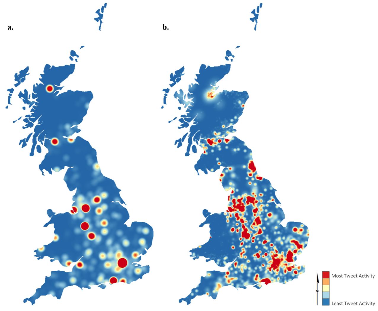
I discussed this problem (in context of Twitter data relating to the 2011 Royal Wedding) of Prince William and Kate Middleton in the Journal of Spatial Information Science, and published a simple algorithm alongside it, which allows false hotspots to be dissipated into realistic patterns based on a weighting surface (population density in this case). In general terms, Weighted Redistribution could be considered an example of a spatial disaggregation algorithm (of which there are many examples), but this one is quite unusual in that it disaggregates data into a surface, rather than smaller aerial units.

Download and read the article, making sure that you understand the problem of False Hotspots and the principles of the Weighted Redistribution algorithm that may be used to solve it.

The Question

Produce your own implementation of my weighted redistribution algorithm and apply it to the provided ‘tweets’ dataset in order to determine which parts of Greater Manchester were most interested in the Royal Wedding, as part of a plan to target advertising during such events.

You will have a random sample of 1,023 level 3 tweets relating to the Royal Wedding that have been geocoded to districts in Greater Manchester. Using these and the weighted redistribution algorithm, you should work out a likely spatial distirbution for Twitter (now called X) activity across Manchester relating to the Royal Wedding.

Produce a 1,000 word report explaining and justifying your implementation of the weighted redistribution algorithm to the level 3 Twitter data in order to produce your map.

The analysis and outputs should be completed entirely in Python using only the libraries provided in the understandinggis environment and the report should include at least one map. You must submit both your code and report.

Make sure that you read this whole document before you start!

The datasets for the Assessment are available in the data/wr/ directory in the repository. This contains:

• data/wr/level3-tweets-subset.shp the tweets themselves.
• data/wr/100m_pop_2019.tif: a weighting surface (simple population density surface at 100m resolution).
• data/wr/gm-districts.shp: polygons representing the districts (level 3) of Greater Manchester to which these tweets were geocoded.

Please note that you are not limited to the data provided, nor are you required to use the provided weighting surface - I would encourage you to include any data that you like to embellish the analytical or cartographic quality of your report (just make saure to add it to your repository).

Contents

• Submission
  • Creating your Assessment 2 Git Repository
• Marking Criteria
• Assessment 1 Hints & Tips
  • Creating a Random Point
  • Code Presentation and AI Use
  • Additional Pointers

1. Submission

   This work must be submitted by 14:00 on Thursday 8^th January 2026.

   You must submit your code and a report of up to up to 1,000 words in length describing the choices that you made in order to create an accurate and efficient algorithm. Code snippets can be used in the report where appropriate (not included in the word count) - but remember that I do not just want a line by line description of your code (that is what your comments are for)!

   ***Note that you must submit your assessment as described here - not having read the below instructions will not be accepted as a reason for late or incorrect submission***

   1. The Code part of your submission must be submitted as a link to your Assessment 2 GitHub Repository (see below), stored under your using your gis-123456789 GitHub account. Submit the HTTPS URL to this form

      The URL is easily accessed by going to your ugis-assessment2 repository on the GitHub website, clicking the the green Code button and selecting the HTTPS tab. It should look something like this: https://github.com/gis-123456789/ugis-assessment2.git).

      Please make sure you submit your own link - not my jonny-huck link or the 123456789 example above!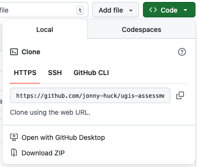

      

   2. The Report part of your submission must be submitted as usual on Canvas. The report should contain the map(s) that you have produced. Submitted files should be named in the format: 123456789.docx or 123456789.pdf etc.

   3. Please check that my user has been successfully added to your GitHub repository (in Collaborators on the website) - if it still says “pending invite” at the time you submit, then please delete the invite and re-send.

   4. This step is optional, but following submission, please consider fill out the AI Policy Survey, which is completely anonymous - this will allow us to make sure that it is as effective as possible.

Creating your Assessment 2 Git Repository

Your Assessment 2 Git Repository should be separate to your main understandinggis repository. As before, you will create this using a template that alrady contains the necessary directory structure and datasets. This is just the same process as you did in Week 1, and for Assessment 1:

First, go to this website to get the Assessment 2 template. Click on the green Use this template button in the top tight and select the option for Create a new repository. Name the repository ugis-assessment2, set visibility to Private and click the green Create Repository button. Follow the process until you have your repository.

Next, click on Settings (at the top of the page) → Collaborators and click Add people.

Type jonny-huck into the search bar and select my user “Jonny Huck” (NOTE: you need to add jonny-huck, not jonnyhuck), then click Invite - this will allow me to be able to access the repository for marking purposes.

Finally, clone the repository into your UGIS/ directory using GitHub Desktop.

You are now ready to start coding your assessment! Don’t forget to commit regularly with informative messages and push to your remote repostory (this is what gets marked, and also provides a backup of your code incase of disaster!).

Marking Criteria

Marks will be given based upon:

1. The quality of the solution (code repository) (60%), comprising:

• Adherence to the AI Policy

• Evidence of proper use of version control (frequent commits and informative messages, assessed through the git log). The assessment of your version control then serves as a multiplier (on a scale of 0-1) for:

  • Detailed comments (remember the rule of thirds), demonstrating a thorough understanding of what you have done - assessed by reading the code - this is the most important part
  • The presentation and elegance of the code - assessed by reading the code
  • The result (i.e., does the solution give the expected answer) - assessed by running the code
  • The efficiency of the solution (i.e., the speed with which your algorithm resolves the problem) - assessed by running the code
  • The robustness of the solution (i.e., the script will not fail if it encounters ’normal’ problems, such as incorrect file paths, missing data, unexpected inputs, and so on) - assessed by running the code

  Accordingly - please be sure that you understand that inadequate version control will severely limit the marks available to you - it is vitally important that you commit frequently with detailed commit messages and that your code contains detailed comments.

1. The quality of the report (40%), comprising:

   • You should explain why Weighted Redistribution is necesssary and how it works, before providing justification for the approaches that you have taken in your implementation, and a discussion around the limitations of your the algorithm and your implementation of it. In all cases, we are looking for you to demonstrate that you have understood both the algorithm and what you have done to implement it. This is not a line by line description of your code (your comments do this), but an explanation of why you made key decisions that contributed to the elegance, efficiency or robustness of this algorithm; and the quality of the map.

   • Throughout, you would expect clear links to the material that we have covered in class as well as the Huck et al. 2015 paper.

   • If you use functions that are not drawn from the practicals, you must explain them in detail and provide references to the associated documentation.

   • The cartographic quality and legibility of the resulting map(s).

   • You must include a Statement on AI Usage, declaring whether you have used Generative AI to help in the production of your submission.

   • Space is limited, so you need to prioritise the most important elements that best demonstrate your understanding.

The key to this is in the name of the course: In both your code and report I want you to demonstrate a clear understanding of what you have done (this is why comments and commit messages are so important in your code)!

References are not mandatory (other than Huck et al. 2015), but may be useful to support your demonstration of underdstanding.

Assessment 2 Hints and Tips

Remember the golden rule: Don’t Panic! You have done everything you need to complete this assessment in the course already, this is just a matter of finding the right bits and putting them together! The pseudocode is given in the paper, so all you have to do is implement it.

As with Assessment 1 - the key is to plan what you are going to do before you start coding - don’t just dive in and hope for the best! All you need to do is keep breaking down each stage into smaller and smaller jobs until you have a clear idea of how the program should look (think about the algorithm).

Everything that you need to be able to do has been covered in the course before, so if you find yourself heading too far off the beaten track, then this is a good clue that you might be overcomplicating things! Remember that you have generic examples of all of the major operations that we have covered available in the Hints page, and the solutions for all of the previous practicals are available on the Solutions page. If you get stuck, you can get help via the forum!

The eagle-eyed of you will note from the paper that I published the original software (written in Java) here. You are welcome to look at it if you want: this is the file with the algorithm in it. However, please do not attempt to simply copy and paste this code and convert it to Python, nor to give it to an AI to translate - this will not result in a good mark! Focus on the approaches that I have taught you in this course to create your own implementation, and remember to maximise efficiency and elegance wherever possible.

Creating a Random Point

In the original version, I used an approach where I selected a random distance and direction from the centroid of polygon, giving a random polar coordinate. You will notice that this is quite different to the approach given in Understanding Distortion, which simply generates a random x and y coordinate based on the bounding box of the feature, giving a random cartesian coordinate.

There are no more or less marks for either approach - though they will give slightly different outputs. My current opinion is that the Understanding Distortion approach is better, so I would recommend using this one over the one I used in the paper.

If, however, you do want to use the Minimium bounding circle approach that I used, then shapely has a convenient function that you can use. Note that there are no more or less marks for either approach.

Code Presentation and AI Use

Presenting neat and tidy code is an important part of Python - one of the key ideas that Guido van Rossum had when creating Python was that code is read much more often than it is written, and so it makes sense to prioritise readability over writability.

Good, tidy, readable code demonstrates that It will demonstrate that you are a competent programmer, and will even help to get you good marks in your assessments! Key elements of well presented code include:

• Follow the Rule of Thirds and make sure that your comments explain exactly what is going on.
• Make sure that variable, function and class names are all descriprive of what they do.
• Use snake_case for variable and function names.
• Make sure your code is well structured, normally:
  1. import statements
  2. functions
  3. main code
• Do not leave in any unnecessary testing material, such as print() statements that do not contribute to the user experience.
• Do not import libraries or functions that you are not using.
• Remember that you MUST adhere to the AI Policy, and you must use proper Version Control throughout your development process, as part of your assessment is your git log. Failing to do either of these things will likely result in a very low mark (see Marking Criteria).

For more guidance on how best to present your code, check out PEP8, the official Style Guide for Python Code.

Additional Pointers

1. Don’t put it off, the longer you give yourself to complete this, the easier you will make it for yourself. Remember that this assignment is about consolidation of your knowledge from the course so far - you should expect to find it challenging, but remember that there is nothing in this assessment that you haven’t done already (or will do…) as part of the course practicals.
2. Read these instructions carefully and in their entirety - particularly around submission - you must submit both your GitHub URL and Report for the submission to count.
3. Don’t underestimate the importance of proper version control - a poor Git log could mean that you can only access a maximum score of 40%.
4. Don’t try to use AI to do it for you - you won’t learn anything, and will likely get a very poor mark.
5. Look back to the lectures and practical material, and make use of the Hints and Solutions pages.
6. Note that you are only undertaking this analysis for a single level, so you can ignore the outer (first) loop described in the pseudocode in the paper (which loops through multiple levels).
7. Be sure to select your parameters (such as \(n\) and \(r\)) for the algorithm carefully - the paper explains how they affect the analysis, so use this knowledge and some experimentation to get the best result for your client - you will definitely want to explain the variables and your selected values to your client.
8. Note that you are only undertaking this analysis for a single level, so you can ignore the outer (first) loop described in the pseudocode in the paper (which loops through multiple levels).
9. Don’t overlook the cartography - it is worth putting some effort into the map to show me that you can use and understand the plotting functions.
10. When explaining what you are doing - remember that I am more interested in the justification (i.e., what you are doing and why) than your implementation (i.e., which library or function you used) - remember that your report is intended to demonstrate a thorough understanding of the Geographical Information Science.
11. If you do feel like you are starting to panic - talk to me!

Good Luck!!