In which we learn to determine whether or not something is visible, as well as speed up our raster processing by replacing geometry with simple graphics algorithms.

Part 1

Last week we began our examination of raster data formats through the creation of a simple flood-fill algorithm. This week we will extend this and learn to calculate visibility - i.e. whether or not something is visible from a given location. Visibility analysis is extremely common in GIS, which makes it all the more surprising how little it is understood by GIS practitioners and decision makers!

One of the interesting things about visibility analysis in GIS is that there are a great deal of different approaches to it, with varying levels of accuracy and speed. A comparison of some common approaches is given by Kaučič and Zalik (2002). This week, we will be using a simplified version of a Viewshed algorithm(written by Jonny Huck) to make it run faster, which is similar to the 8WS approach described in the paper.

One of the key features of this approach is that we will once again exploit working in image space in order to allow us to replace complex geometric calculations with simple graphics algorithms in order make our code more efficient (just as we did with the flood fill algorithm last time). Many of these algorithms were created in the early days of computer graphics, and so are designed to be extremely efficient (as computer power was so limited at the time).

Specifically, we will use two algorithms:

• Bresenham’s Line algorithm, which draws a line across a surface from one pixel to another.
• Midpoint Circle algorithm (a.k.a. Bresenham’s Circle Algorithm), which draws a circle of a given size (in pixels) around a given pixel.

These algorithms are extremely efficient because they allow us to draw lines and circles simply using the + and - operators, completely avoiding the use of trigonometry, which would be much more complex (see here to remind yourself how this would work using point offsets).

We will not be implementing the Bresenham’s Line or Midpoint Circle algorithms directly - instead we will use the implementations that are provided by the draw module of the scikit-image library, which contains a range of functions for image processing in Python. This will allow us to focus on the details of the visibility calculation itself (which we cover in Part 2). However, if you want to know more about these algorithms, you can read about both of them in the original paper by Bresenham (1965).

Because we can apply algorithms like those provided in scikit-image, it is quite a good rule of thumb for raster-based algorithms that the more work you can do in Image Space, the faster your code could be. Also remember the golden rule to help avoid errors - try to work entirely in either image space or coordinate space - avoid mixing and matching if you can!

Take a look at the drawing algorithms available in scikit-image they might come in handy in the future…

CRS

As with last week, our data are already projected to the British National Grid (EPSG: 27700) - a local conformal projected CRS designed by Ordnance Survey for general use in Great Britain. For this reason, we do not need to select a CRS this week, as we know that this is an acceptable CRS for use in our area of interest (the Lake District).

Setting up a new Raster Layer

Last week, we learned how to open a raster layer and make a blank copy of it using the zeros() function from numpy. Let’s set one of those up now using the same dataset (Lake District, Cumbria, UK), just as we did last week:

from numpy import zeros
from rasterio import open as rio_open
from rasterio.plot import show as rio_show
from matplotlib.pyplot import subplots, savefig
from matplotlib.colors import LinearSegmentedColormap

# open the elevation data file
with rio_open("../data/helvellyn/Helvellyn-50.tif") as dem:

    # read the data out of band 1 in the dataset
    dem_data = # COMPLETE THIS LINE

    # create a new 'band' of raster data the same size
    output = # COMPLETE THIS LINE

# plot the dataset
fig, my_ax = subplots(1, 1, figsize=(16, 10))

# add the DEM
rio_show(
  dem_data,
  ax=my_ax,
  transform = dem.transform,
)
# add the drawing layer
rio_show(
    output,
    ax=my_ax,
    transform=dem.transform,
    cmap = LinearSegmentedColormap.from_list('binary_viewshed', [(0, 0, 0, 0), (1, 0, 0, 0.5)], N=2)
    )
savefig('./out/bresenham.png', bbox_inches='tight')

Create a new file called bresenham.py in your week8 directory, add the above snippet, making sure to complete the missing lines, and run it

Remember that we used LinearSegmentedColormap from the matplotlib.colors library to create our own colormap, in which values of 0 are set to transparent black (0, 0, 0, 0), and values of 1 are set to a different colour. Last week we chose a shade of blue (to represent flood water), this week we will use semi- red (1, 0, 0, 0.5)

Make sure that you understand the above (if not, refer back to the last practical!) and then run your code

If all goes to plan, you should have a map of the DEM (because the new image is all 0s, and so completely transparent):

Drawing to your new Raster Layer

Drawing a Point

Now we have an transparent layer laying perfectly over our map, and we know that any pixels that we set to 1 will appear as red.

As with last week, let’s start by drawing a point. Remember that the steps for this are:

1. Convert the coordinates from coordinate space (x,y) to image space (row,col) using the .index() function of the rasterio dataset object.
2. Set the pixel at this location in your output surface to 1

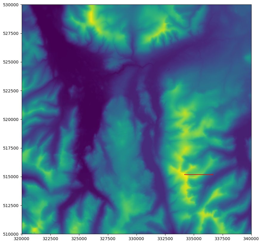
Using the above and your knowledge from last week, see if you can draw a point at 334170, 515165. Though it is perfectly possible to do this in a single line of code, I want you to use two lines of code (one for each step above), storing the image space coordinates in variables called row and col - this is because we are going to use these values again in a moment.

If all went to plan, you should see the summit of Helvellyn go red (as with before - it is one tiny pixel, so you need to look closely!):

Great! Now we have drawn a point, let’s try drawing a line…

Drawing a Line (using Bresenham’s Line Algorithm)

We could easily draw a line by working out which cells to colour using trigonometry, but we will be using the (much more efficient) Bresenham’s Line Algorithm. We will use it via the line() function from the draw module of scikit-image.

This is a simple function that gives us a list of pixel locations (given in image space) that describe a line between two locations (also given in image space). We will demonstrate this by drawing a 50 pixel line due east from our existing point location. line has 4 arguments: the first two are the coordinates of the cell in which the line should start, and the second two are the coordinates of the cell in which the line should finish (both coordinates are in image space, and so row, col).

Add the below snippets to your code and run it to see the results

from skimage.draw import line

print(line(row, col, row, col+50))

If all went to plan, you should see something like this (I have shortened this using ellipses ... - yours should have a tuple of two numpy arrays each containing 51 numbers):

(array([296, 296, 296, ..., 296, 296, 296]), array([283, 284, 285, ..., 331, 332, 333]))

numpy arrays (a type of Python collection provided by the numpy library) are similar to a list, but with more restrictions (e.g. they can only store data of a single type) and more member functions. Here we have a tuple (another type of Python Collection, with which you are already familiar) of two arrays: one array contains the row coordinates, and the other contains the column coordinates. This is great, but would be more useful if the coordinates were paired up. Fortunately, numpy has us covered once again, with the column_stack function, which does exactly this:

from numpy import column_stack

print(column_stack(line(row, col, row, col+50)))

Add the above import statement to your code (remembering that you can combine it with an existing one…), and replace your print statement with the above one.

You should now be looking at something like this (again I have shortened this using ellipses ... - yours should have a list of 50 lists each containing 2 numbers):

[[296 283]
 [296 284]
 [296 285]
 ...
 [296 331]
 [296 332]
 [296 333]]

Much better! Now we have a single array in which each item is a pair of coordinates (in image space) describing a pixel that is part of the line.

Make sure that you understand what column_stack does - if you are not sure, ask!

Now all that remains is to loop through each of these coordinate pairs and update the value at that location in the output surface to 1:

Loop through each coordinate pair (r, c) returned by this statement and set the output to 1 at that location, run your code and see what the result is

If all has gone to plan, you should be looking at something like this:

If so, then great!! On we go…

Drawing a Circle (using The Midpoint Circle Algorithm)

Finally, let’s add a circle in as well, we will draw one with a 50px radius around our point:

from skimage.draw import circle_perimeter

circle_perimeter(row, col, 50)

Implement the above snippets - you will need to pass the result to column_stack (just as above) and set each cell in the resulting list to 1

Run your code

You should now be looking at something like this:

If so, well done! You can now successfully draw points, lines and circles to a raster - with no geometry in sight!

Part 2

Before we get stuck in with understanding viewsheds, let’s do a bit of setup:

Create a file called week8.py in your week8 folder.

Open "../data/helvellyn/Helvellyn-50.tif", using the variable d to represent the rasterio dataset, and extracting the first (and only) band of the raster as dem_data

Set a location for the origin of the viewshed using the below snippet

# set origin for viewshed
x0, y0 = 332000, 514000

In a moment, we will create a viewshed() function.

In order to allow us to test it, add the function call in the below snippet to your code:

# calculate the viewshed
output = viewshed(x0, y0, 5000, 1.8, 100, dem_data, d)

Now we’re ready to start…

The viewshed() Function

As you saw in the lecture, our viewshed algorithm works by calculating a circle (using the Midpoint Circle Algorithm), and then calculating a line of sight to each location on the circle, updating each cell in the line as we go. Each of these two steps will be represented by a function - we will start by making the viewshed() function, and then move on to line_of_sight() later on.

Create a new function called viewshed() with 7 arguments as listed below:

1. x0, the x coordinate (in coordinate space) of the point from which we will calculate the viewshed
2. y0, the y coordinate (in coordinate space) of the point from which we will calculate the viewshed
3. radius_m, the radius (in metres) of the viewshed
4. observer_height, the height (in metres) of the observer for whom the viewshed will be calculated
5. target_height, the height (in metres) of the target (e.g. a wind turbine) to which the viewshed will be calculated
6. dem_data, the DEM data (the band from the rasterio dataset)
7. d, the rasterio dataset containing the DEM dataset

The viewshed() function will work out the endpoint for each line of sight (each cell in the circle) and then call the line_of_sight() function to work out the visibility of each point on a line from the origin to that location.

The first thing that it will do, however, is to convert everything from coordinate space to image space - it is important to do this straight away, as otherwise you can get mixed up, which is a common way to introduce errors into your code when working with rasters!

Convert x0 and y0 to image space, storing the results as r0 and c0 for the row and column value respectively.

Now that we have this - we have the opportunity to make our code more robust, by checking that the specified location is actually within the area covered by the dataset. We could have done this using the bounding box of the raster dataset and a within query using the coordinate space coordinates, but as above it is much simpler to do this in image space, and simply use the between operator to see if the coordinates are larger than 0 and smaller than the width/height of the dataset. If this is not the case (note how we are using the not operator here to invert the results of the conditional statement) we simply print a message to the user and gracefully exit the program.

from sys import exit

	# make sure that we are within the dataset
	if not 0 <= r0 < d.height or not 0 <= c0 < d.width:
		print(f"Sorry, {x0, y0} is not within the elevation dataset.")
		exit()

Make sure that you understand how the above statement works and then add the above snippets to your code at the appropriate locations

One snag when working in image space is that we often need to know the size of each cell, in order to be able to convert it to a distance. For example, the 50 pixel line that we drew above is rather meaningless, unless we know that each cell represents 50m on the ground, meaning that the line is

As we saw last week, we can retrieve the resolution of the dem dataset using the .res property, which returns a tuple containing the x and y resolution. For our purposes, datasets generally have a single resolution for both directions (i.e. the cells are square), so we can simply take the first of the values (that for x) as “the resolution” with dem.res[0].

Add the below snippet to convert the radius_m to image space (from metres to pixels) by dividing it by the resolution of the dataset

	# convert the radius (m) to pixels
	radius_px = int(radius_m / d.res[0])

Now we know the starting location and radius of the viewshed, we are just missing one key bit of information: the starting height of the viewshed - by which I mean the elevation of the origin location + the observer height. To get this, we simply need to read the elevation from the DEM and add it to the observer height. Here is how we do that:

	# get the observer height (above sea level)
	height0 = dem_data[(r0, c0)] + observer_height

Make sure that you understand the above and add it to your code

Add a print() statement to see what the elevation is at our chosen start point, run the code to get the result

(it should be about 180m). Now we are nearly ready to start our viewshed:

Create an output raster surface at the same dimensions as the dem dataset

Set the origin of the viewshed to 1 (as the observer can definitely see the cell in which they are stood)

All we need to do now is calculate our circle, and pass each cell to the line_of_sight()function, before returning our output dataset to be added to the map:

# get pixels in the perimeter of the viewshed
for r, c in column_stack(circle_perimeter(r0, c0, radius_px*3)):

	# calculate line of sight to each pixel, pass output and get a new one back each time
	#output = line_of_sight(r0, c0, height0, r, c, target_height, radius_px, dem_data, d, output)
  pass

# return the resulting viewshed
return output

The above should be self explanatory - just be sure to note that I have tripled the size of radius_px to increase the line density and make sure that we don’t miss any cells in our analysis (as explained in the lecture)! As you can see, each call passes the necessary information to line_of_sight(), which takes the current version of output as an argument, updates visible cells on that line to 1, and then returns the result. The effect is that output is overwritten with a more complete version every iteration of the loop, until every line has been assessed and the viewshed is complete.

Also of note here is the use of the pass statement - this just tells it to do nothing inside the loop, without it you would get an error because there is no code inside the loop (an empty code block like this would be interpreted as an error)

Make sure that you understand the above snippet, and add it to your code

Check that your code runs without error. If so, un-comment the line that begins output = ... from the above snippet and delete the pass statement.

If so, great - now we can get down to business with our calculation…

The line_of_sight() Function

As you will remember from the lecture, as we move along a line of sight, we check each cell in turn, and work out the \(\Delta y /\Delta x\). If it is bigger than any we have seen previously, then the cell is visible. If it is not bigger, then the cell is invisible - simple!

Create a new function called line_of_sight() with 10 arguments as listed below:

1. r0, the row coordinate of the pixel at the start of the line (in image space)
2. c0, the column coordinate of the pixel at the start of the line (in image space)
3. height0, elevation+height of the pixel at the start of the line (in metres)
4. r1, the row coordinate of the pixel at the end of the line (in image space)
5. c1, the column coordinate of the pixel at the end of the line (in image space)
6. height1, the height of the pixel at the end of the line (in metres)
7. radius, the radius of the viewshed (in pixels - image space)
8. dem_data, the DEM data (the band from the rasterio dataset)
9. d, the rasterio dataset containing the DEM dataset (and the Affine Transformation Matrix, for converting between image and coordinate space)
10. output, the output dataset to which the new data will be added

We will therefore loop along the line from (r0,c0) to (r1,c1), and calculate \(\Delta y /\Delta x\) at each cell. If it is greater than any previous \(\Delta y /\Delta x\) value, then the cell is visible, and so we set the value to 1 in the output dataset. If not, we leave it at 0.

To get started, we will initialise a variable to hold the largest \(\Delta y /\Delta x\) so far, and then we will loop through each cell in our line (ignoring the first one, which we know is visible because our observer is stood in it…). Because the value could be positive or negative (depending on whether we are looking uphill or downhill), we will initialise our tracking variable to negative infinity:

# init variable for biggest dydx so far (starts at -infinity)
max_dydx = -float('inf') 	

# loop along the pixels in the line (excluding the first one)
for r, c in column_stack(line(r0, c0, r1, c1))[1:]:

Note the use of list slicing to exclude the first element from the loop (see the Hints Page if you can’t remember how this works).

Add the above snippet to your code

Inside the loop, we will firstly calculate \(\Delta x\):

Use Pythagoras (you can use the hypot function if you prefer…) to work out the distance (in pixels) between (r0,c0) (the origin point) and (r,c) (the current point) - store the result in a variable called dx

Add the below snippet to stop the loop when it gets to the end of the desired radius (this is necessary because we used a larger radius to calculate the endpoint in order to increase the line density) OR when we hit the end of the dataset (which is always necessary)

		# if we go too far, or go off the edge of the data, stop looping
		if dx > radius or not 0 <= r < d.height or not 0 <= c < d.width:
			break

Temporarily add a print() statement so that you can see the distances - remember to remove this once you have verified that it works!

Next, we just need to work out the \(\Delta y /\Delta x\) value - which we do twice (once for the base of the object that we are looking for, and once for the tip). This is because, when assessing the visibility of the object for this cell, we need to use the tip (as the object will actually be located there); but when we are testing the visibility of the object further down the line, then we want to account for the ground level at that location (as the object will not be there to block visibility).

		# calculate the current value for dy / dx
		base_dydx = (dem_data[(r, c)] - height0) / dx
		tip_dydx = (dem_data[(r, c)] + height1 - height0) / dx

Make sure that you understand that (if not, ask!) and add the above snippet to your code

Make sure that it runs without error

Finally, we just need to test if this \(\Delta y /\Delta x\) was the biggest so far, and if so update the cell in the output surface accordingly. We can then return the freshly edited output to the viewshed() function, which will add the rest of the lines of sight to it, before returning it to out main code block where we can draw the result!

Add the below snippet to your code to complete the line_of_sight() function:

		# if the tip dydx is bigger than the previous max, it is visible
		if (tip_dydx > max_dydx):
			output[(r, c)] = 1

		# if the base dydx is bigger than the previous max, update
		max_dydx = max(max_dydx, base_dydx)

	# return updated output surface
	return output

Make sure that it runs without error

Drawing your map

If that all runs without error - then there is a very good chance that you are successfully calculating a viewshed! To check - we can draw it to a map - there is nothing new here (we did it all last week or in Part 1), so I will give this in a single block (I will stick with the default 'viridis' colour ramp, but feel free to change it to another one!):

from math import floor, ceil
from geopandas import GeoSeries
from shapely.geometry import Point
from matplotlib.lines import Line2D
from matplotlib.patches import Patch
from matplotlib.colors import Normalize
from matplotlib.cm import ScalarMappable
from rasterio.plot import show as rio_show
from matplotlib.pyplot import subplots, savefig
from matplotlib_scalebar.scalebar import ScaleBar
from matplotlib.colors import LinearSegmentedColormap

	# output image
	fig, my_ax = subplots(1, 1, figsize=(16, 10))
	my_ax.set_title("Viewshed Analysis")

	# draw dem
	rio_show(
		dem_data,
		ax=my_ax,
		transform = d.transform,
		cmap = 'viridis',
		)

	# draw dem as contours
	rio_show(
		dem_data,
		ax=my_ax,
		contour=True,
		transform = d.transform,
		colors = ['white'],
		linewidths = [0.5],
		)

	# add viewshed
	rio_show(
		output,
		ax=my_ax,
		transform=d.transform,
		cmap = LinearSegmentedColormap.from_list('binary_viewshed', [(0, 0, 0, 0), (1, 0, 0, 0.5)], N=2)
		)

	# add origin point
	GeoSeries(Point(x0, y0)).plot(
		ax = my_ax,
		markersize = 60,
		color = 'black',
		edgecolor = 'white'
		)

	# add a colour bar
	fig.colorbar(ScalarMappable(norm=Normalize(vmin=floor(dem_data.min()), vmax=ceil(dem_data.max())), cmap='viridis'), ax=my_ax, pad=0.01)

	# add north arrow
	x, y, arrow_length = 0.97, 0.99, 0.1
	my_ax.annotate('N', xy=(x, y), xytext=(x, y-arrow_length),
		arrowprops=dict(facecolor='black', width=5, headwidth=15),
		ha='center', va='center', fontsize=20, xycoords=my_ax.transAxes)

	# add scalebar
	my_ax.add_artist(ScaleBar(dx=1, units="m", location="lower right"))

	# add legend for point
	my_ax.legend(
		handles=[
			Patch(facecolor=(1, 0, 0, 0.5), edgecolor=None, label=f'Visible Area'),
			Line2D([0], [0], marker='o', color=(1,1,1,0), label='Viewshed Origin', markerfacecolor='black', markersize=8)
		], loc='lower left')

	# save the result
	savefig('./out/7.png', bbox_inches='tight')
	print("done!")

Add the above snippet to your code at the appropriate location and run it

If all has gone to plan, you should have something like this:

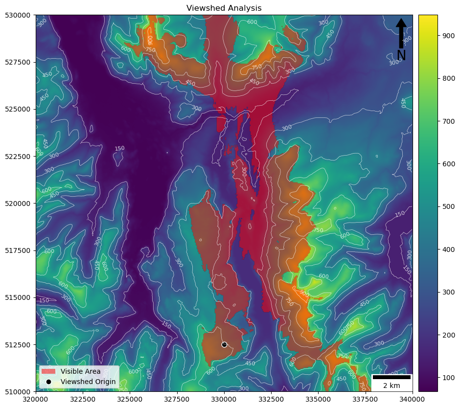
(where the red represents the area visible from the black dot)

If so then congratulations - you have calculated your own viewshed from scratch!!

Try adjusting your origin point and radius (coordinates are shown on the axes) to see if the pattern of visibility matches with your expectations. You will notice how the chosen radius is extremely important, and that increasing the radius affects the speed of execution.

A little more…

If you want to go a little further, we can add one more function to account for atmospheric refraction and the curvature of the Earth. This can be achieved with a relatively simple equation:

where:

\(height_{adjusted}\) is the resulting (adjusted) height

\(height\) is the original (un-adjusted) height

\(\Delta x\) is the distance in metres - multiply by the resolution of the dataset in metres (50) to convert from pixels - you can obtain this from the rasterio dataset with dem_input.res[0])

\(D\) is the diameter of the Earth in metres

\(R\) is the atmospheric refraction coefficient

Add a new function using the snippet below, and complete it to reflect the above equation

Edit your base_dydx and tip_dydx lines in line_of_sight() to make use of this function

def adjust_height(height, distance, earth_diameter=12740000, refraction_coefficient=0.13):
	"""
	* Adjust the apparant height of an object at a certain distance, accounting for the
	* 	curvature of the earth and atmospheric refraction
	"""
	return 

You will note that we have used some optional arguments in this function (earth_diameter=12740000, refraction_coefficient=0.13). When I do this, I can either choose to define these values or just ignore them and accept the default values. For example, I could set all of the values as normal:

adjust_height(height, distance, 12800000, 0.15)

…or I can just ignore them and accept the defaults:

adjust_height(height, distance)

…or I can use a named argument and just set one of them, and accept the default for the other (which allows for them not to be in the right order because I have missed one):

adjust_height(height, distance, refraction_coefficient=0.15)